Gradient-based optimization of fluid flows

Note

All examples are expected to run from the examples/<example_name> directory of the Tesseract-JAX repository.

In this example, you will learn how to:

1. Build a Tesseract that wraps a differentiable simulator from JAX-CFD.

2. Access its endpoints via Tesseract-JAX’s apply_tesseract() function.

3. Perform gradient-based optimization of the fluid simulation (via scipy.optimize.minimize), using the Tesseract as a differentiable simulator.

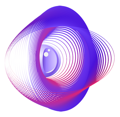
The goal of this application is to find initial conditions for which the final fluid flow is close to this image (the Pasteur Labs logo):

from IPython.display import Image

Image(filename="pl.png", width=200)

# Install additional requirements for this notebook
%pip install -r requirements.txt -q

[notice] A new release of pip is available: 25.0 -> 25.0.1
[notice] To update, run: pip install --upgrade pip
Note: you may need to restart the kernel to use updated packages.

Step 1: Build + serve JAX-CFD Tesseract

cfd-tesseract is a differentiable Navier-Stokes solver based on JAX-CFD that is wrapped in a Tesseract.

Here is its apply function, as defined in cfd_tesseract/tesseract_api.py:

def cfd_fwd(
    v0: jnp.ndarray,
    density: float,
    viscosity: float,
    inner_steps: int,
    outer_steps: int,
    max_velocity: float,
    cfl_safety_factor: float,
    domain_size_x: float,
    domain_size_y: float,
) -> tuple[jax.Array, jax.Array]:
    """Compute the final velocity field using the semi-implicit Navier-Stokes equations.

    Args:
        v0: Initial velocity field.
        density: Density of the fluid.
        viscosity: Viscosity of the fluid.
        inner_steps: Number of solver steps for each timestep.
        outer_steps: Number of timesteps steps.
        max_velocity: Maximum velocity.
        cfl_safety_factor: CFL safety factor.
        domain_size_x: Domain size in x direction.
        domain_size_y: Domain size in y direction.

    Returns:
        Final velocity field.
    """
    vx0 = v0[..., 0]
    vy0 = v0[..., 1]
    bc = cfd.boundaries.HomogeneousBoundaryConditions(
        (
            (cfd.boundaries.BCType.PERIODIC, cfd.boundaries.BCType.PERIODIC),
            (cfd.boundaries.BCType.PERIODIC, cfd.boundaries.BCType.PERIODIC),
        )
    )

    # reconstruct grid from input
    grid = cfd.grids.Grid(
        vx0.shape, domain=((0.0, domain_size_x), (0.0, domain_size_y))
    )

    vx0 = cfd.grids.GridArray(vx0, grid=grid, offset=(1.0, 0.5))
    vy0 = cfd.grids.GridArray(vy0, grid=grid, offset=(0.5, 1.0))

    # reconstruct GridVariable from input
    vx0 = cfd.grids.GridVariable(vx0, bc)
    vy0 = cfd.grids.GridVariable(vy0, bc)
    v0 = (vx0, vy0)

    # Choose a time step.
    dt = cfd.equations.stable_time_step(
        max_velocity, cfl_safety_factor, viscosity, grid
    )

    # Define a step function and use it to compute a trajectory.
    step_fn = cfd.funcutils.repeated(
        cfd.equations.semi_implicit_navier_stokes(
            density=density, viscosity=viscosity, dt=dt, grid=grid
        ),
        steps=inner_steps,
    )
    rollout_fn = cfd.funcutils.trajectory(step_fn, outer_steps)
    _, trajectory = jax.device_get(rollout_fn(v0))
    vxn = trajectory[0].array.data[-1]
    vyn = trajectory[1].array.data[-1]
    return jnp.stack([vxn, vyn], axis=-1)

To build the Tesseract, we use the tesseract command line tool.

%%bash
# Build CFD Tesseract so we can use it below
tesseract build cfd-tesseract/

?25l [i] Building image ...
⠼ Processing
 [i] Built image sha256:7632fcec515b, ['jax-cfd:latest']

["jax-cfd:latest"]

To interact with the Tesseract, we use the Python SDK from tesseract_core to load the built image and start a server container.

from tesseract_core import Tesseract

cfd_tesseract = Tesseract.from_image("jax-cfd")
cfd_tesseract.serve()

Step 2: Test forward evaluation with Tesseract-JAX

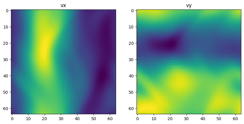
Let’s set up the Tesseract with Tesseract-JAX and test a simple forward evaluation. First, we’ll define an initial guess for the velocity field over a grid. The resulting vx and vy give our horizontal and vertical velocity fields, respectively.

# Import necessary libraries
import jax
import jax.numpy as jnp
import jax_cfd.base as cfd
import matplotlib.animation as animation
import matplotlib.pyplot as plt
import numpy as np
from PIL import Image as PILImage
from scipy.optimize import minimize
from tqdm import tqdm

from tesseract_jax import apply_tesseract

# Set up the CFD simulation parameters
seed = 0
size = 64
max_velocity = 3.0
domain_size_x = jnp.pi * 2
domain_size_y = jnp.pi * 2

bc = cfd.boundaries.HomogeneousBoundaryConditions(
    (
        (cfd.boundaries.BCType.PERIODIC, cfd.boundaries.BCType.PERIODIC),
        (cfd.boundaries.BCType.PERIODIC, cfd.boundaries.BCType.PERIODIC),
    )
)

grid = cfd.grids.Grid((size, size), domain=((0, domain_size_x), (0, domain_size_y)))
v0 = cfd.initial_conditions.filtered_velocity_field(
    jax.random.PRNGKey(seed), grid, max_velocity
)
vx, vy = v0

params = {
    "density": 1.0,
    "viscosity": 0.01,
    "inner_steps": 25,
    "outer_steps": 30,
    "max_velocity": max_velocity,
    "cfl_safety_factor": 0.5,
    "domain_size_x": domain_size_x,
    "domain_size_y": domain_size_y,
}

# Define initial velocity field
v0 = np.stack([np.array(vx.array.data), np.array(vy.array.data)], axis=-1)


# Define the Tesseract function
def cfd_tesseract_fn(v0):
    return apply_tesseract(cfd_tesseract, inputs=dict(v0=v0, **params))


# Apply Tesseract to the initial velocity field
outputs = cfd_tesseract_fn(v0)

Using the results of the forward pass, we can set up a basic approach for visualising our velocity field. We’ll use matplotlib to show the \(x\) and \(y\) components of the velocity as heatmaps.

vxn = outputs["result"][..., 0]
vyn = outputs["result"][..., 1]

fig, ax = plt.subplots(1, 2, figsize=(10, 5))
ax[0].imshow(vxn, cmap="viridis")
ax[0].set_title("vx")
ax[1].imshow(vyn, cmap="viridis")
ax[1].set_title("vy")

Text(0.5, 1.0, 'vy')

Next we define a vorticity function for later use (recalling that vorticity is the curl of the flow velocity, ie. \(\omega = \nabla \times \mathbf{v}\)).

def vorticity(vxn, vyn):
    vxn = cfd.grids.GridArray(vxn, grid=grid, offset=(1.0, 0.5))
    vyn = cfd.grids.GridArray(vyn, grid=grid, offset=(0.5, 1.0))

    # reconstrut GridVariable from input
    vxn = cfd.grids.GridVariable(vxn, bc)
    vyn = cfd.grids.GridVariable(vyn, bc)

    # differntiate
    _, dvx_dy = cfd.finite_differences.central_difference(vxn)
    dvy_dx, _ = cfd.finite_differences.central_difference(vyn)

    return dvy_dx.data - dvx_dy.data

Step 3: Optimize the initial state so the fluid evolves into the Pasteur Labs logo

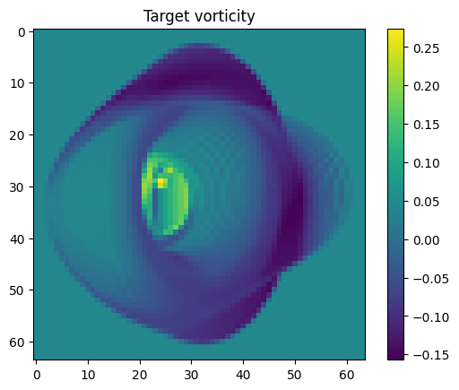
Now we want to perform an actual optimization. Our goal is to find an initial state \(v_0\), such that the vorticity of the final state \(v_N\) resembles the Pasteur Labs logo.

Let’s start by loading in our logo.

img = plt.imread("pl.png")
img = img.mean(axis=-1)
img = PILImage.fromarray((img * 255).astype(np.uint8))
img_shape_y, img_shape_x = img.size

img = img.resize((size, size))
img = np.array(img).astype(np.float32) / 255.0

# normalize around 0
img = img - img.mean()

plt.imshow(img, cmap="viridis")
plt.colorbar()
plt.title("Target vorticity")

Text(0.5, 1.0, 'Target vorticity')

We define the loss function, which additionally ensures physical realism of the initial condition by penalizing the flow’s divergence.

def mse(x, y):
    return jnp.mean((x - y) ** 2)


def divergence(vxn, vyn):
    vxn = cfd.grids.GridArray(vxn, grid=grid, offset=(1.0, 0.5))
    vyn = cfd.grids.GridArray(vyn, grid=grid, offset=(0.5, 1.0))

    # reconstruct GridVariable from input
    vxn = cfd.grids.GridVariable(vxn, bc)
    vyn = cfd.grids.GridVariable(vyn, bc)

    return cfd.finite_differences.divergence([vxn, vyn]).data


def loss_fn(v0_flat, target=img, xlen=grid.shape[0]):
    total_len = len(v0_flat)
    ylen = (total_len // 2) // xlen
    v0x = v0_flat[: total_len // 2].reshape(xlen, ylen)
    v0y = v0_flat[total_len // 2 :].reshape(xlen, ylen)

    div = divergence(v0x, v0y)

    vn = cfd_tesseract_fn(v0=jnp.stack([v0x, v0y], axis=-1))["result"]

    vxn = vn[..., 0]
    vyn = vn[..., 1]

    vort = vorticity(vxn, vyn)

    # add divergence penalty term to ensure the field is divergence free
    return mse(vort, target) + 0.05 * mse(div, 0.0)

Finally, we perform the optimization with the help of the L-BFGS-B optimizer from scipy.optimize.minimize. This exploits the fact that the loss function is fully differentiable with respect to the initial velocity field \(v_0\).

Executing this cell can take a few minutes.

v0_field = cfd.initial_conditions.filtered_velocity_field(
    jax.random.PRNGKey(221), grid, max_velocity
)
v0_flat = np.array([vx.array.data, vy.array.data]).flatten()
grad_fn = jax.jit(jax.value_and_grad(loss_fn))

max_iter = 400
with tqdm(total=max_iter) as pbar:
    i = 0

    def callback(intermediate_result):
        global i
        i += 1
        pbar.set_postfix(loss=f"{intermediate_result.fun:.4f}")
        pbar.update(1)

    opt = minimize(
        grad_fn,
        v0_flat,
        method="L-BFGS-B",
        jac=True,
        callback=callback,
        options={"maxiter": max_iter},
    )

print(f"Optimisation converged after {i} iterations")

 27%|██▋       | 109/400 [01:56<05:11,  1.07s/it, loss=0.0006]

Optimisation converged after 109 iterations

Finally, we generate a video of the optimization result. For this, we change the number of outer loops of the cfd simulation to 1, which enables us to save the state of the simulation at each time step.

v0_flat = opt.x
xlen = grid.shape[0]
ylen = grid.shape[1]
v0x = v0_flat[: xlen * ylen].reshape(xlen, ylen)
v0y = v0_flat[xlen * ylen :].reshape(xlen, ylen)
v0 = jnp.stack([v0x, v0y], axis=-1)

trajectory = []
vi = v0.copy()

params_2 = params.copy()
params_2.update({"outer_steps": 1})


def cfd_tesseract_fn(v0):
    res = apply_tesseract(cfd_tesseract, inputs=dict(v0=v0, **params_2))
    return res["result"]


for _ in range(30):
    vi = cfd_tesseract_fn(vi)

    vxn = vi[..., 0]
    vyn = vi[..., 1]

    vort = vorticity(vxn, vyn)

    trajectory.append(vort)

# repeat last frame a few times
trajectory.extend([vort] * 10)


fig = plt.figure()

ims = []
for vort in trajectory:
    im = plt.imshow(vort, cmap="plasma", animated=True)
    # remove axis
    plt.axis("off")
    ims.append([im])

ani = animation.ArtistAnimation(fig, ims, interval=100, blit=True, repeat_delay=1000)
plt.close(fig)

ani.save("/tmp/vorticity.gif", writer="pillow", fps=10)
Image(filename="/tmp/vorticity.gif", embed=True)

And voilà! We have successfully optimized the initial velocity field to evolve into the Pasteur Labs logo, using differentiable programming with Tesseract-JAX and JAX-CFD.

# Tear down Tesseract after use to prevent resource leaks
cfd_tesseract.teardown()