Steady conduction in a slab

H Heat transfer Generated 2026-11-06 17:21 UTC 12 plots

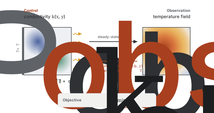
Invert for the conductivity field of a slab from its temperature, differentiating through a steady heat-conduction solve.

Inferring conductivity from temperature. Given the temperature field of a heated slab, where is the material conductive? We answer this inverse problem by differentiating through a steady heat-conduction solve.

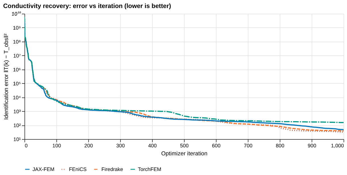
The conductivity of a quasi-2D slab follows the SIMP law (\(p=3\)) \(k_\text{eff}(\rho) = k_\min + (k_\max - k_\min)\,\rho^3\) in the element density \(\rho\). The optimization experiment recovers a two-Gaussian density field from the temperature it produces, starting from a uniform field and minimizing \(\lVert T(\rho) - T_\text{target} \rVert^2\) with L-BFGS. The forward and gradient experiments compare solvers on the thermal compliance \(C = \oint_\Gamma q_n\,T\,d\Gamma\), the work done by the heat flux on the temperature field, and on its sensitivity to \(\rho\). Two further gradient experiments check the derivative of a temperature misfit with respect to a volumetric heat source \(f(\mathbf{x})\).

How these results were produced

These are example results, produced automatically on GitHub-hosted runners and refreshed on every release. Each solver runs on its intended device: GPU-capable solvers on a Tesla T4 GPU node, CPU-only solvers (OpenFOAM, deal.II, FEniCS, Firedrake, TopOpt.jl) on a separate CPU node. Each benchmark job has its virtual machine to itself, but the hardware and the load on the host can change from run to run, so wall-clock times vary. Read them for relative scaling between solvers rather than as absolute timings. Accuracy and gradient metrics change little across hardware, although float32 arithmetic is not identical across devices and chaotic rollouts amplify small discrepancies. For numbers that reflect your setup, run the benchmark yourself on your target hardware.

Boundary conditions

Quasi-2D heated slab on domain \([0,2]\times[0,1]\) (a single HEX8 layer, \(n_z=1\)). The slab thickness \(L_z\) scales with the in-plane element size (\(L_z = L_x/n_x\)) so the elements stay roughly cubic under refinement, keeping the linear system well-conditioned; \(Q_\text{total}\) is thus a flux per unit slab depth. Dirichlet: all nodes at \(x=0\) held at \(T=0\) (fixed temperature). Neumann (uniform): uniform heat flux \(Q_\text{total}\) over the right face (\(x=2\)). Neumann (hot-spot): flux concentrated on the central \(1/3\) stripe in \(y\) (\(L_y/3 \le y \le 2L_y/3\)) at the right face, used by the physical-laws check.

Checks

The results overview explains the columns and states.

Solver	Forward	Gradient	Optimization	Forward cost	VJP cost	Time to plateau	Peak memory	Effort
GPU solversForward and VJP, multiples of the fastest GPU solver
JAX-FEM	✓Pass	✓Pass	✓Pass	—	—	—	—	L0
torch-fem	✓Pass	✓Pass	✓Pass	—	—	—	—	L0
CPU solversForward and VJP at N=1024, multiples of the fastest CPU solver
FEniCS	✓Pass	✓Pass	✓Pass	14.3 sfastest	30.5 sfastest	2.1 minfastest	4.67 GiB	L3
Firedrake	✓Pass	✓Pass	✓Pass	—	—	—	—	L0
deal.II	✓Pass	—Not supported	—Not supported	20.1 s1.4×	—	—	1.87 GiB	L0

Flags and exclusions (12)

• Firedrake on cost/spatial_cost: not run
• Firedrake on cost/temporal_cost: not run
• Firedrake on cost/vjp_cost/by_N: not run
• Firedrake on cost/vjp_cost/by_steps: not run
• JAX-FEM on cost/spatial_cost: not run
• JAX-FEM on cost/temporal_cost: not run
• JAX-FEM on cost/vjp_cost/by_N: not run
• JAX-FEM on cost/vjp_cost/by_steps: not run
• torch-fem on cost/spatial_cost: not run
• torch-fem on cost/temporal_cost: not run
• torch-fem on cost/vjp_cost/by_N: not run
• torch-fem on cost/vjp_cost/by_steps: not run

Not supported (1 solver)

• deal.II, 7 experiments. The deal.II thermal tesseract is forward-only. It exposes no AD path (no VJP endpoint, no differentiable inputs), so cost/vjp and gradient experiments are categorically out of scope.; The deal.II thermal tesseract exposes no AD path, and conductivity recovery (gradient-based ρ updates that minimize the misfit to a target temperature field) requires a differentiable identification-error output.

Initial conditions

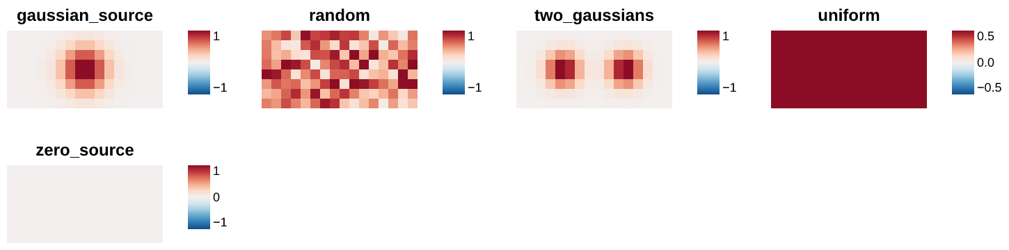
The initial conditions and fields that this setup’s experiments start from. They are plotted without running any solver.

Settings

gaussian_source

{
  "nx": 16,
  "ny": 8,
  "nz": 1,
  "amplitude": 1.0,
  "cx": 0.5,
  "cy": 0.5,
  "sigma": 0.2
}

random

{
  "rho_0": 0.5,
  "noise": 0.3,
  "nx": 16,
  "ny": 8,
  "nz": 1,
  "seed": 0
}

two_gaussians

{
  "nx": 16,
  "ny": 8,
  "nz": 1
}

uniform

{
  "rho_0": 0.5,
  "nx": 16,
  "ny": 8,
  "nz": 1
}

zero_source

{
  "nx": 16,
  "ny": 8,
  "nz": 1
}

Forward

Is the prediction right? Forward experiments compare each solver’s output with a trusted reference, an analytic solution where one exists, and the other solvers.

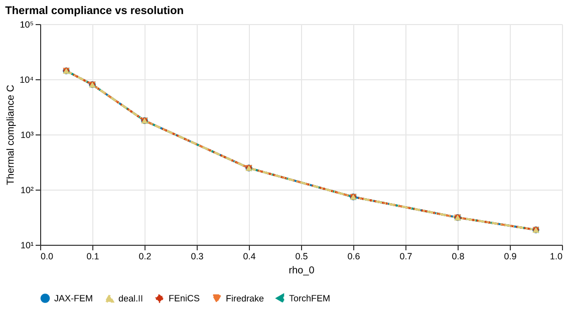
Agreement between solvers

Thermal compliance \(C\) vs uniform element density \(\rho_0\) at fixed \(N\); compares solvers on a log scale.

Settings

Sweeps rho_0 ∈ {0.05, 0.1, 0.2, 0.4, 0.6, 0.8, 0.95}

{
  "ic": {
    "name": "uniform",
    "seed": 0
  },
  "physics": {
    "nx": 16,
    "ny": 8,
    "nz": 1,
    "Lx": 2.0,
    "Ly": 1.0,
    "Q_total": 1.0,
    "rho_0": 0.05
  },
  "sweep": {
    "key": "rho_0",
    "values": [
      0.05,
      0.1,
      0.2,
      0.4,
      0.6,
      0.8,
      0.95
    ]
  }
}

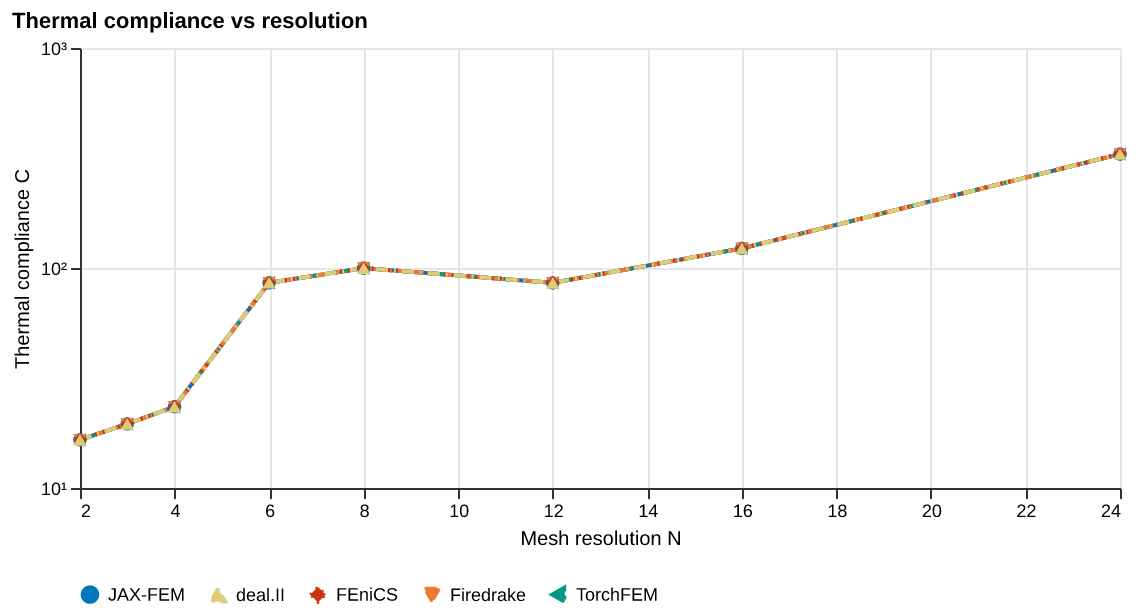
Agreement with the reference

Thermal compliance \(C\) vs mesh resolution \(N\) with random density; compares the solvers across refinements.

Settings

Sweeps N ∈ {2, 3, 4, 6, 8, 12, 16, 24}

{
  "ic": {
    "name": "random",
    "seed": 0
  },
  "physics": {
    "N": 2,
    "nz": 1,
    "Lx": 2.0,
    "Ly": 1.0,
    "Q_total": 1.0
  },
  "sweep": {
    "key": "N",
    "values": [
      2,
      3,
      4,
      6,
      8,
      12,
      16,
      24
    ]
  }
}

Conservation and decay laws

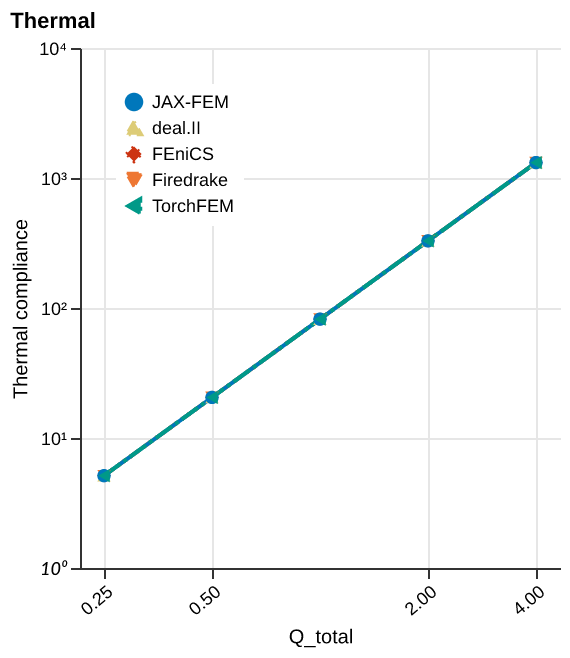
Thermal compliance \(C\) vs total heat flux \(Q_\mathrm{total}\) at fixed \(N\) and \(\rho_0\) with a hot-spot BC; shown on log-log axes.

Settings

Sweeps Q_total ∈ {0.25, 0.5, 1.0, 2.0, 4.0}

{
  "ic": {
    "name": "uniform",
    "seed": 0
  },
  "physics": {
    "N": 16,
    "nz": 1,
    "Lx": 2.0,
    "Ly": 1.0,
    "rho_0": 0.5,
    "hot_spot": true,
    "Q_total": 0.25
  },
  "sweep": {
    "key": "Q_total",
    "values": [
      0.25,
      0.5,
      1.0,
      2.0,
      4.0
    ]
  },
  "diagnostics": {
    "thermal_compliance": "<callable _get_thermal_compliance>"
  }
}

Agreement with the reference (heat source)

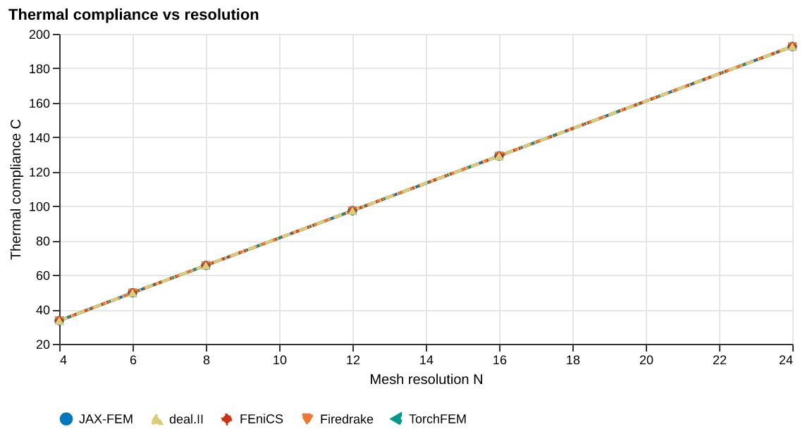
Thermal compliance \(C\) vs mesh resolution \(N\) with a Gaussian source field; compares solvers across refinements.

Settings

Sweeps N ∈ {4, 6, 8, 12, 16, 24}

{
  "ic": {
    "name": "gaussian_source"
  },
  "physics": {
    "N": 4,
    "nz": 1,
    "Lx": 2.0,
    "Ly": 1.0,
    "rho_0": 0.5,
    "ic_field": "source"
  },
  "sweep": {
    "key": "N",
    "values": [
      4,
      6,
      8,
      12,
      16,
      24
    ]
  }
}

Linearity in the heat source

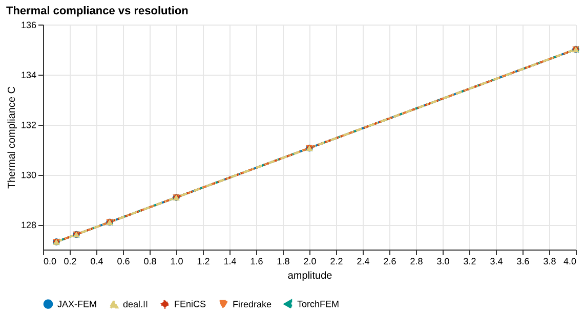
Thermal compliance \(C\) vs source amplitude at fixed mesh; compares solvers on log-log axes.

Settings

Sweeps amplitude ∈ {0.1, 0.25, 0.5, 1.0, 2.0, 4.0}

{
  "ic": {
    "name": "gaussian_source"
  },
  "physics": {
    "nx": 16,
    "ny": 8,
    "nz": 1,
    "Lx": 2.0,
    "Ly": 1.0,
    "rho_0": 0.5,
    "ic_field": "source",
    "amplitude": 0.1
  },
  "sweep": {
    "key": "amplitude",
    "values": [
      0.1,
      0.25,
      0.5,
      1.0,
      2.0,
      4.0
    ]
  }
}

Results by solver

Solver	Mean rel. error
deal.II	1.74e-08
FEniCS	1.74e-08
Firedrake	1.74e-08
JAX-FEM	1.74e-08
torch-fem	1.74e-08

From Agreement between solvers.

Cost

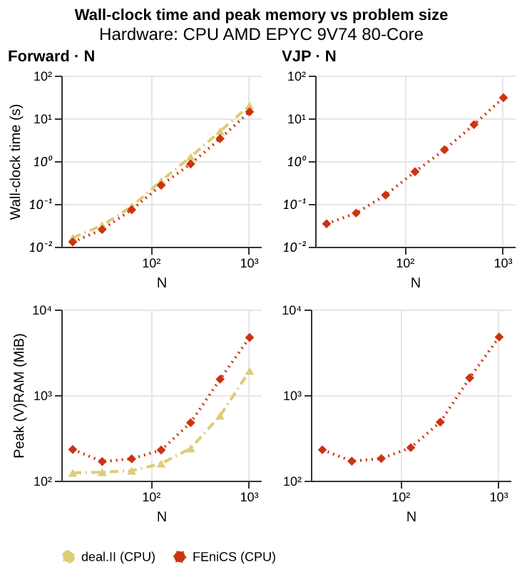
What does it cost? Wall-clock time and peak memory of the forward and VJP passes as the problem size \(N\) and the number of steps grow. See the note on how these results were produced before reading absolute numbers.

Settings

spatial_cost

Sweeps nx ∈ {16, 32, 64, 128, 256, 512, 1024}

{
  "physics": {
    "Lx": 2.0,
    "Ly": 1.0,
    "Q_total": 1.0,
    "rho_0": 0.5,
    "steps": 1,
    "nx": 16
  },
  "cost": {
    "n_trials": 10
  },
  "sweep": {
    "key": "nx",
    "values": [
      16,
      32,
      64,
      128,
      256,
      512,
      1024
    ]
  }
}

temporal_cost

Sweeps steps ∈ {1}

{
  "physics": {
    "Lx": 2.0,
    "Ly": 1.0,
    "Q_total": 1.0,
    "rho_0": 0.5,
    "nx": 64,
    "steps": 1
  },
  "cost": {
    "n_trials": 10
  },
  "sweep": {
    "key": "steps",
    "values": [
      1
    ]
  }
}

Results by solver

Solver	Device	Forward time (N=1024)	Forward first call	VJP time (N=1024)	VJP / forward	Forward peak memory	VJP peak memory
FEniCS	CPU	14.3 s	45.7 s	30.5 s	2.13×	4.6 GiB	4.67 GiB
deal.II	CPU	20.1 s	20.6 s	—	—	1.87 GiB	—

From Forward cost across resolution.

Gradient

Is the gradient right? Gradient experiments compare each solver’s AD or adjoint gradient with finite differences, in magnitude (relative \(L^2\) error) and direction (cosine similarity).

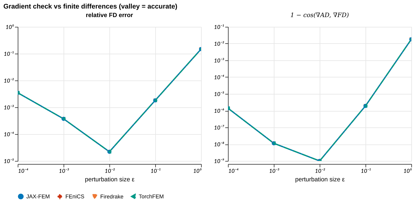
Gradient against finite differences

FD gradient error vs step size \(\varepsilon\) (U-curves), AD/FD direction cosine, and gradient magnitude field panels.

Settings

{
  "ic": {
    "name": "random",
    "seed": 0
  },
  "physics": {
    "nx": 8,
    "ny": 4,
    "nz": 1,
    "Lx": 2.0,
    "Ly": 1.0,
    "Q_total": 1.0
  },
  "fd": {
    "eps_values": [
      1.0,
      0.1,
      0.01,
      0.001,
      0.0001
    ],
    "n_dirs": 6
  }
}

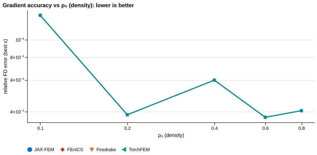
Gradient accuracy across the control parameter

Gradient norm, best-\(\varepsilon\) FD error, AD/FD direction cosine, and U-curves vs element density \(\rho_0\).

Settings

Sweeps rho_0 ∈ {0.1, 0.2, 0.4, 0.6, 0.8}

{
  "ic": {
    "name": "uniform",
    "seed": 0
  },
  "physics": {
    "nx": 8,
    "ny": 4,
    "nz": 1,
    "Lx": 2.0,
    "Ly": 1.0,
    "Q_total": 1.0,
    "rho_0": 0.1
  },
  "fd": {
    "eps_values": [
      1.0,
      0.1,
      0.01,
      0.001,
      0.0001
    ],
    "n_dirs": 6
  },
  "sweep": {
    "key": "rho_0",
    "values": [
      0.1,
      0.2,
      0.4,
      0.6,
      0.8
    ]
  }
}

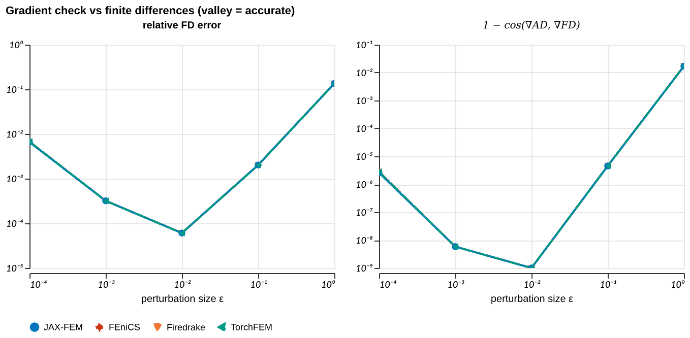
Gradient with respect to the heat source

FD gradient error vs \(\varepsilon\), AD/FD direction cosine, and gradient field panels for d(identification_error)/d(source).

Settings

{
  "ic": {
    "name": "gaussian_source"
  },
  "ic_key": "source",
  "output_key": "identification_error",
  "physics": {
    "nx": 8,
    "ny": 4,
    "nz": 1,
    "Lx": 2.0,
    "Ly": 1.0,
    "rho_0": 0.5,
    "target_from_two_gaussians": true,
    "ic_field": "source"
  },
  "fd": {
    "eps_values": [
      1.0,
      0.1,
      0.01,
      0.001,
      0.0001
    ],
    "n_dirs": 6
  }
}

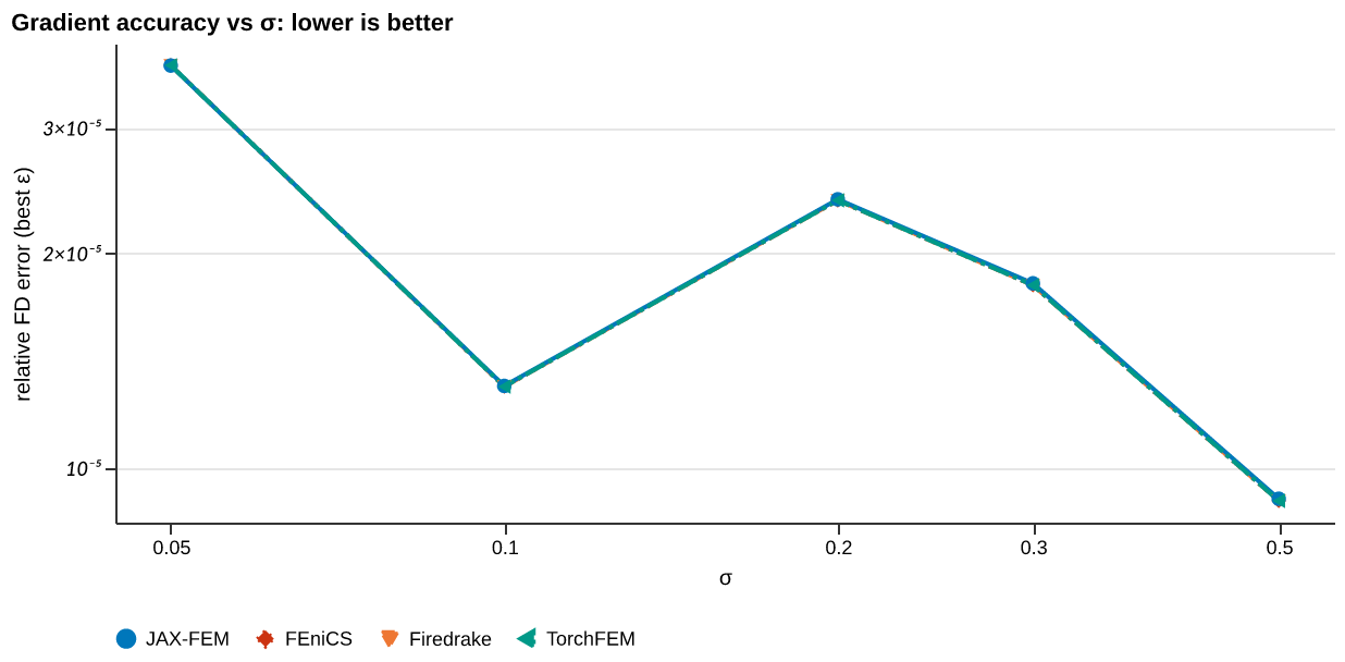
Heat-source gradient across source width

Gradient norm, best-\(\varepsilon\) FD error, AD/FD direction cosine, and U-curves vs source width \(\sigma\).

Settings

Sweeps sigma ∈ {0.05, 0.1, 0.2, 0.3, 0.5}

{
  "ic": {
    "name": "gaussian_source"
  },
  "ic_key": "source",
  "output_key": "identification_error",
  "physics": {
    "nx": 16,
    "ny": 8,
    "nz": 1,
    "rho_0": 0.5,
    "target_from_two_gaussians": true,
    "ic_field": "source"
  },
  "fd": {
    "eps_values": [
      0.1,
      0.01,
      0.001,
      0.0001
    ],
    "n_dirs": 4
  },
  "sweep": {
    "key": "sigma",
    "values": [
      0.05,
      0.1,
      0.2,
      0.3,
      0.5
    ],
    "ic_sweep": true
  }
}

Results by solver

Solver	Best-ε FD error	1 − cosine
FEniCS	1.83e-05	2.21e-10
Firedrake	1.83e-05	2.21e-10
JAX-FEM	1.83e-05	2.21e-10
torch-fem	1.83e-05	2.21e-10

From Gradient against finite differences.

Optimization

Can you optimize through it? Optimization experiments run a gradient-based optimizer on each solver’s own gradients. A gradient can pass the finite-difference check and still fail to drive an optimization loop.

Conductivity recovery (L-BFGS)

Optimisation traces (loss vs iteration) and recovered conductivity fields vs the two-Gaussian ground truth, using L-BFGS.

Settings

{
  "ic": {
    "name": "uniform",
    "seed": 0
  },
  "physics": {
    "nx": 16,
    "ny": 8,
    "nz": 1,
    "Lx": 2.0,
    "Ly": 1.0,
    "rho_0": 0.5,
    "Q_total": 1.0,
    "compliance_key": "identification_error",
    "penalty_weight": 0.0,
    "x_min": 0.001,
    "snap_interval": 10,
    "target_rho_from_two_gaussians": true
  },
  "optim": {
    "max_iters": 1000
  },
  "optimizer": "bfgs"
}

Results by solver

Solver	Final error	Iterations to plateau	Time to plateau
FEniCS	3.12e+01	792	2.1 min
Firedrake	3.87e+01	—	—
JAX-FEM	4.79e+01	—	—
torch-fem	1.53e+02	—	—

From Conductivity recovery (L-BFGS).