Periodic box

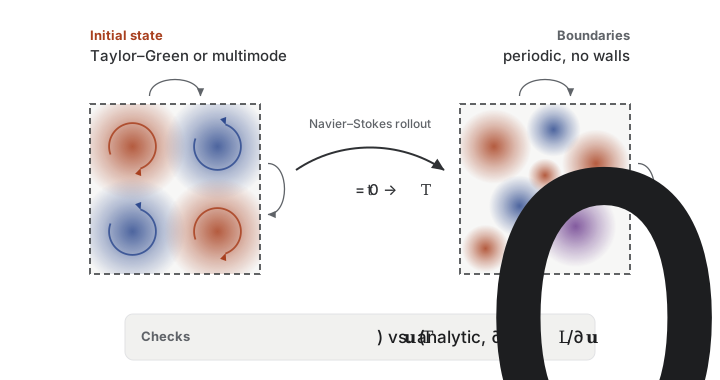
F2 Navier–Stokes (2D) Generated 2026-11-06 17:21 UTC 11 plots

Forward accuracy against the analytic Taylor–Green solution, and how gradients hold up as the rollout lengthens and the flow becomes chaotic, in a 2D box without walls.

Incompressible fluid flow in 2D. We solve and differentiate through the 2D incompressible Navier–Stokes equations \(\partial_t \mathbf{u} + (\mathbf{u}\cdot\nabla)\mathbf{u} = -\nabla p + \nu\,\nabla^2\mathbf{u}\), \(\nabla\cdot\mathbf{u}=0\), with the kinematic viscosity \(\nu\) as the primary control parameter. The problem has three setups: a doubly periodic box, a channel flow past a cylinder, and a forced Kolmogorov flow.

The nonlinear advection term \(\nabla\cdot(\mathbf{u}\otimes\mathbf{u})\) transfers energy across scales. At low \(\nu\) the flow develops turbulent cascades and a positive Lyapunov exponent. Long-horizon gradients then become exponentially sensitive to perturbations, so backpropagation through the simulation is hardest in this regime.

How these results were produced

These are example results, produced automatically on GitHub-hosted runners and refreshed on every release. Each solver runs on its intended device: GPU-capable solvers on a Tesla T4 GPU node, CPU-only solvers (OpenFOAM, deal.II, FEniCS, Firedrake, TopOpt.jl) on a separate CPU node. Each benchmark job has its virtual machine to itself, but the hardware and the load on the host can change from run to run, so wall-clock times vary. Read them for relative scaling between solvers rather than as absolute timings. Accuracy and gradient metrics change little across hardware, although float32 arithmetic is not identical across devices and chaotic rollouts amplify small discrepancies. For numbers that reflect your setup, run the benchmark yourself on your target hardware.

Boundary conditions

Doubly periodic square domain \([0, 2\pi]^2\) (the flow wraps around at every edge), with incompressibility \(\nabla\cdot\mathbf{u}=0\) enforced by a pressure projection at each time step.

Checks

The results overview explains the columns and states.

Solver	Forward	Gradient	Forward cost	VJP cost	Peak memory	Effort
GPU solversForward and VJP at N=256, multiples of the fastest GPU solver, measured on Tesla T4
jax-cfd	Pass	Pass3 of 4 run	40.1 ms1.2×	85.6 ms1.1×	512 MiB	L0
Warp-NS	Pass	Pass3 of 4 run	99.8 ms2.9×	407 ms5.0×	4 MiB	L2
XLB modified setup	Pass	Pass3 of 4 run	266 ms7.7×	1.49 s18×	8 GiB	L2
INS.jl	Pass	Pass3 of 4 run	280 ms8.1×	986 ms12×	32 MiB	L0
PhiFlow	Pass	Pass3 of 4 run	22 s640×	68.3 s840×	1.09 GiB	L3
Exponax	Flagged	Pass3 of 4 run	34.4 msfastest	81.3 msfastest	256 MiB	L2
PICT	Flagged	Pass	4.99 s145×	10.5 s129×	4.97 GiB	L0
CPU solversForward and VJP at N=256, multiples of the fastest CPU solver
OpenFOAM	Flagged	Not supported	7.72 sfastest	—	528 MiB	L0

Solvers differ in how general they are. Exponax and jax-cfd do not run Channel flow past a cylinder. Exponax, INS.jl, OpenFOAM, PhiFlow, Warp-NS, XLB and jax-cfd do not run Forced Kolmogorov flow.

Modified setups (1)

These solvers run a substitute for part of the setup, so their checks hold for the modified setup.

XLB: Sub-steps each step to bound the Mach number. Effect: LBM ties the time step to the grid through the lattice Mach number, so XLB runs k times the prescribed number of steps (k = 9 at N = 256 on the 2-D box), and its cost includes them. Without sub-stepping the Taylor-Green case ran at Ma of about 0.88, with errors 84 to 114x the peer median.

Flags and exclusions (9)

jax-cfd on gradient/analytic_check_nu: not run
Warp-NS on gradient/analytic_check_nu: not run
XLB on gradient/analytic_check_nu: not run
INS.jl on gradient/analytic_check_nu: not run
PhiFlow on gradient/analytic_check_nu: not run
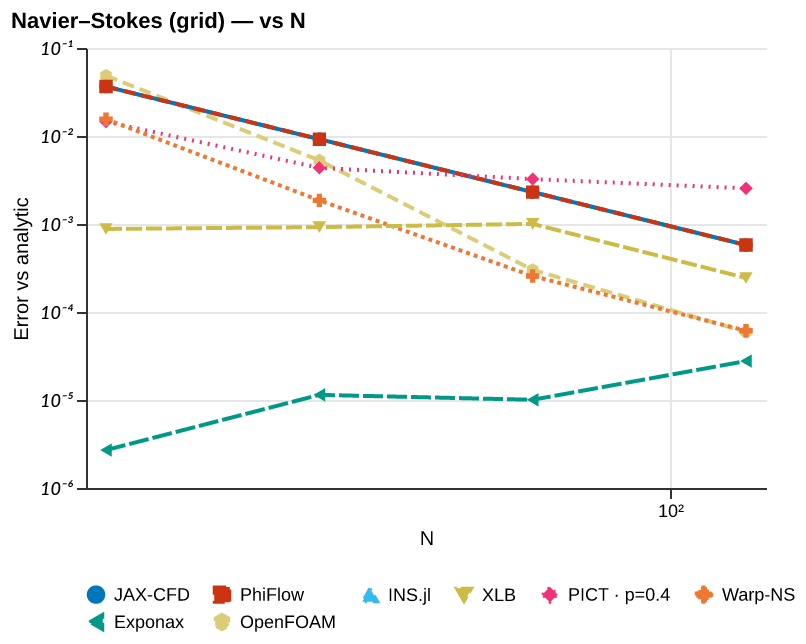
Exponax on forward/baseline: flagged. error converges at order -1.46 in N, below min_order=0.8 (explained: the Taylor–Green vortex is a single Fourier mode, which a spectral method represents exactly on every grid, so Exponax's error is float32 round-off from the first step. Round-off grows with the number of grid points and steps rather than shrinking with the grid spacing, so no positive order can be observed)
Exponax on gradient/analytic_check_nu: not run
PICT on forward/baseline: flagged. error converges at order 0.35 in N, below min_order=0.8 (explained: PICT runs PISO with its default two pressure correctors, and its momentum predictor carries no pressure gradient. The splitting error this leaves scales with ν·dt/dx², which grows as the grid is refined at fixed CFL, so the error levels off on the finest grids and the observed order drops. More correctors remove the floor at a multiple of the wall time and reverse-mode memory)
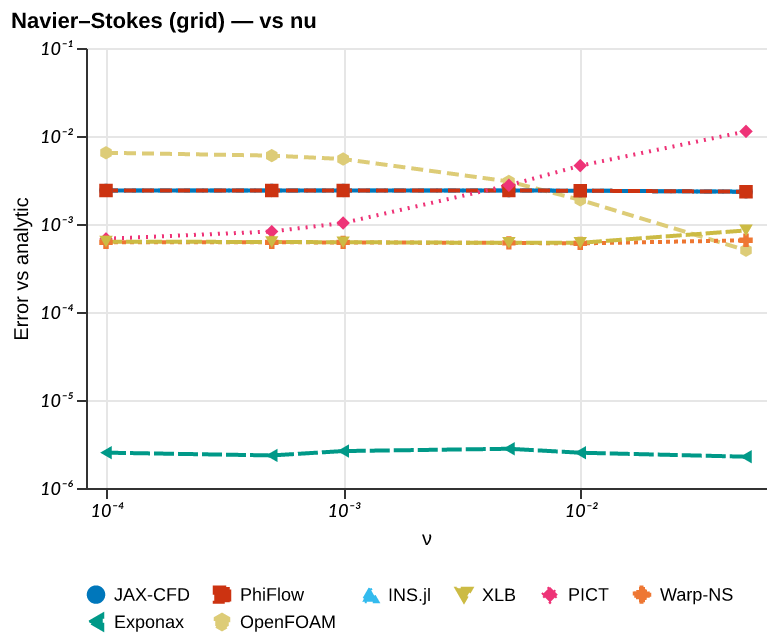
OpenFOAM on forward/tgv_nu_sweep: flagged. error 0.00645 at sweep=0.0001 is 4.2× peer median (0.00154); threshold k=3.0 (explained: OpenFOAM stores velocity at cell centres and makes only the face fluxes divergence-free. In the Taylor–Green vortex, advection is a gradient at twice the vortex's wavenumber, which the pressure cancels exactly. Most of OpenFOAM's error is a compressive component at that wavenumber in the cell-centred velocity. The staggered and spectral solvers have none of it, the other solvers at most a tenth of it. It is second order in the grid spacing, grows with the simulated time and the vortex's amplitude, and changes little with the timestep. It shrinks as the viscosity grows, so it stands out only at the lowest viscosities)

Not supported (1 solver)

OpenFOAM, 11 experiments. OpenFOAM has no VJP to benchmark; OpenFOAM is non-differentiable (C++, no AD path); DAFoam/OpenFOAM-AD exist but are not deployed in this tesseract

Initial conditions

The initial conditions and fields that this setup’s experiments start from. They are plotted without running any solver.

Settings

dfg_inflow

{
  "resolution": 20
}

flat_inflow

{
  "N": 64,
  "U": 0.5
}

multimode

{
  "N": 64
}

rest

{
  "N": 64
}

tgv

{
  "N": 64
}

uniform

{
  "N": 64,
  "U": 1.0
}

Forward

Is the prediction right? Forward experiments compare each solver’s output with a trusted reference, an analytic solution where one exists, and the other solvers.

Agreement with the reference

Relative error vs grid resolution \(N\) against the analytic TGV solution at \(t=1.28\), refining space and time together at a fixed CFL number. The legend gives each solver’s observed order of accuracy \(p\).

Settings

Sweeps N ∈ {16, 32, 64, 128}

{
  "ic": {
    "name": "tgv",
    "seed": 0
  },
  "physics": {
    "N": 16,
    "nu": 0.05,
    "dt": 0.01,
    "steps": 128,
    "cfl_N_base": 128
  },
  "sweep": {
    "key": "N",
    "values": [
      16,
      32,
      64,
      128
    ]
  }
}

Accuracy across viscosity (Taylor–Green)

Relative error vs viscosity \(\nu\) for each solver at a fixed TGV initial condition.

Settings

Sweeps nu ∈ {0.0001, 0.0005, 0.001, 0.005, 0.01, 0.05}

{
  "ic": {
    "name": "tgv",
    "seed": 42
  },
  "physics": {
    "N": 64,
    "dt": 0.05,
    "steps": 20,
    "nu": 0.0001
  },
  "sweep": {
    "key": "nu",
    "values": [
      0.0001,
      0.0005,
      0.001,
      0.005,
      0.01,
      0.05
    ]
  }
}

Results by solver

Solver	Mean rel. error
Exponax	2.51e-06
Warp-NS	6.20e-04
XLB	6.57e-04
PhiFlow	2.39e-03
jax-cfd	2.39e-03
INS.jl	2.39e-03
PICT	3.53e-03
OpenFOAM	3.89e-03

From Accuracy across viscosity (Taylor–Green).

Cost

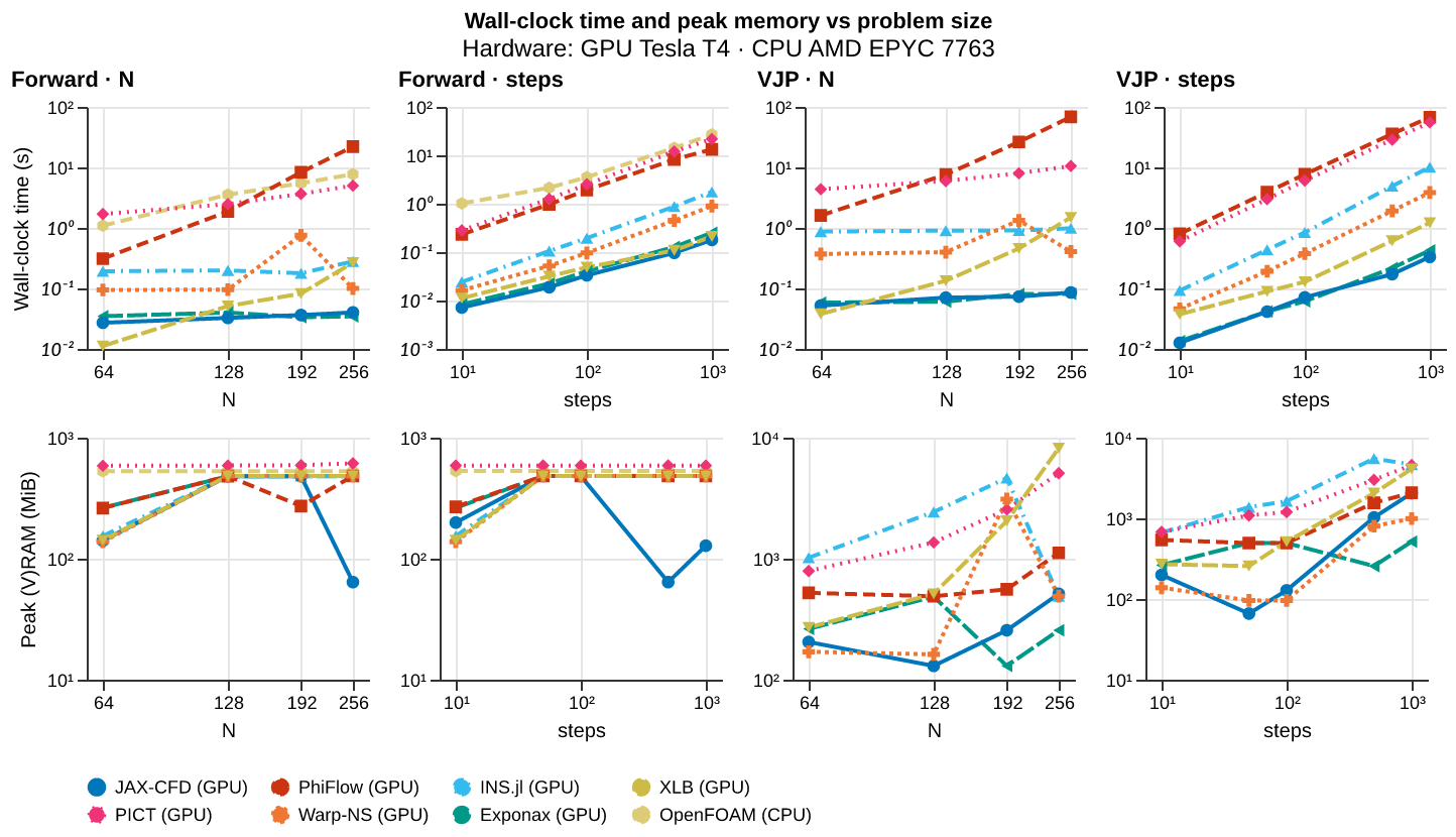
What does it cost? Wall-clock time and peak memory of the forward and VJP passes as the problem size \(N\) and the number of steps grow. See the note on how these results were produced before reading absolute numbers.

Settings

spatial_cost

Sweeps N ∈ {64, 128, 192, 256}

{
  "physics": {
    "nu": 0.01,
    "dt": 0.01,
    "steps": 100,
    "N": 64
  },
  "cost": {
    "n_trials": 3
  },
  "sweep": {
    "key": "N",
    "values": [
      64,
      128,
      192,
      256
    ]
  }
}

temporal_cost

Sweeps steps ∈ {10, 50, 100, 500, 1000}

{
  "physics": {
    "nu": 0.01,
    "dt": 0.01,
    "N": 128,
    "steps": 10
  },
  "cost": {
    "n_trials": 3
  },
  "sweep": {
    "key": "steps",
    "values": [
      10,
      50,
      100,
      500,
      1000
    ]
  }
}

Results by solver

Solver	Device	Forward time (N=256)	Forward first call	VJP time (N=256)	VJP / forward	Forward peak memory	VJP peak memory
Exponax	GPU	0.0344 s	1.31 s	0.0813 s	2.36×	2 MiB	256 MiB
jax-cfd	GPU	0.0401 s	1.36 s	0.0856 s	2.13×	64 MiB	512 MiB
Warp-NS	GPU	0.0998 s	7.8 s	0.407 s	4.08×	4 MiB	4 MiB
XLB	GPU	0.266 s	1.43 s	1.49 s	5.58×	0 MiB	8 GiB
INS.jl	GPU	0.28 s	0.29 s	0.986 s	3.53×	32 MiB	32 MiB
PICT	GPU	4.99 s	4.99 s	10.5 s	2.11×	612 MiB	4.97 GiB
PhiFlow	GPU	22 s	32.8 s	68.3 s	3.1×	30 MiB	1.09 GiB
OpenFOAM	CPU	7.72 s	7.9 s	—	—	528 MiB	—

From Forward cost across resolution.

Gradient

Is the gradient right? Gradient experiments compare each solver’s AD or adjoint gradient with finite differences, in magnitude (relative \(L^2\) error) and direction (cosine similarity).

Settings

analytic_check

Sweeps nu ∈ {0.001, 0.005, 0.01, 0.02, 0.05}

{
  "ic": {
    "name": "tgv",
    "seed": 0
  },
  "physics": {
    "N": 32,
    "dt": 0.05,
    "steps": 20,
    "nu": 0.001
  },
  "reference": "<callable _tgv_analytic_grad>",
  "sweep": {
    "key": "nu",
    "values": [
      0.001,
      0.005,
      0.01,
      0.02,
      0.05
    ]
  },
  "project": "<callable project_divergence_free>"
}

analytic_check_nu

Sweeps nu ∈ {0.001, 0.005, 0.01, 0.02, 0.05}

{
  "ic": {
    "name": "tgv",
    "seed": 0
  },
  "physics": {
    "N": 32,
    "dt": 0.05,
    "steps": 20,
    "nu": 0.001
  },
  "reference": "<callable _tgv_analytic_dJ_dnu>",
  "sweep": {
    "key": "nu",
    "values": [
      0.001,
      0.005,
      0.01,
      0.02,
      0.05
    ]
  },
  "wrt": "viscosity"
}

chain_fd_check

{
  "physics": {
    "N": 64,
    "dt": 0.01,
    "steps": 10,
    "intervals": 16,
    "offset": 0.01,
    "nu": 0.002,
    "forcing_wavenumber": 4,
    "forcing_amplitude": 1.0,
    "linear_drag": 0.1
  },
  "fd": {
    "eps_values": [
      1.0,
      0.1,
      0.01
    ],
    "n_dirs": 8
  }
}

fd_check

{
  "ic": {
    "name": "multimode",
    "seed": 42
  },
  "physics": {
    "N": 16,
    "nu": 0.001,
    "dt": 0.05,
    "steps": 20
  },
  "fd": {
    "eps_values": [
      5.0,
      1.0,
      0.1,
      0.01,
      0.001,
      0.0001
    ],
    "n_dirs": 20
  }
}

horizon_sweep

Sweeps steps ∈ {5, 10, 20, 40, 80, 160, 320}

{
  "ic": {
    "name": "multimode",
    "seed": 42
  },
  "physics": {
    "N": 16,
    "nu": 0.001,
    "dt": 0.05,
    "steps": 5
  },
  "fd": {
    "eps_values": [
      1.0,
      0.1,
      0.01,
      0.001
    ],
    "n_dirs": 8
  },
  "sweep": {
    "key": "steps",
    "values": [
      5,
      10,
      20,
      40,
      80,
      160,
      320
    ]
  }
}

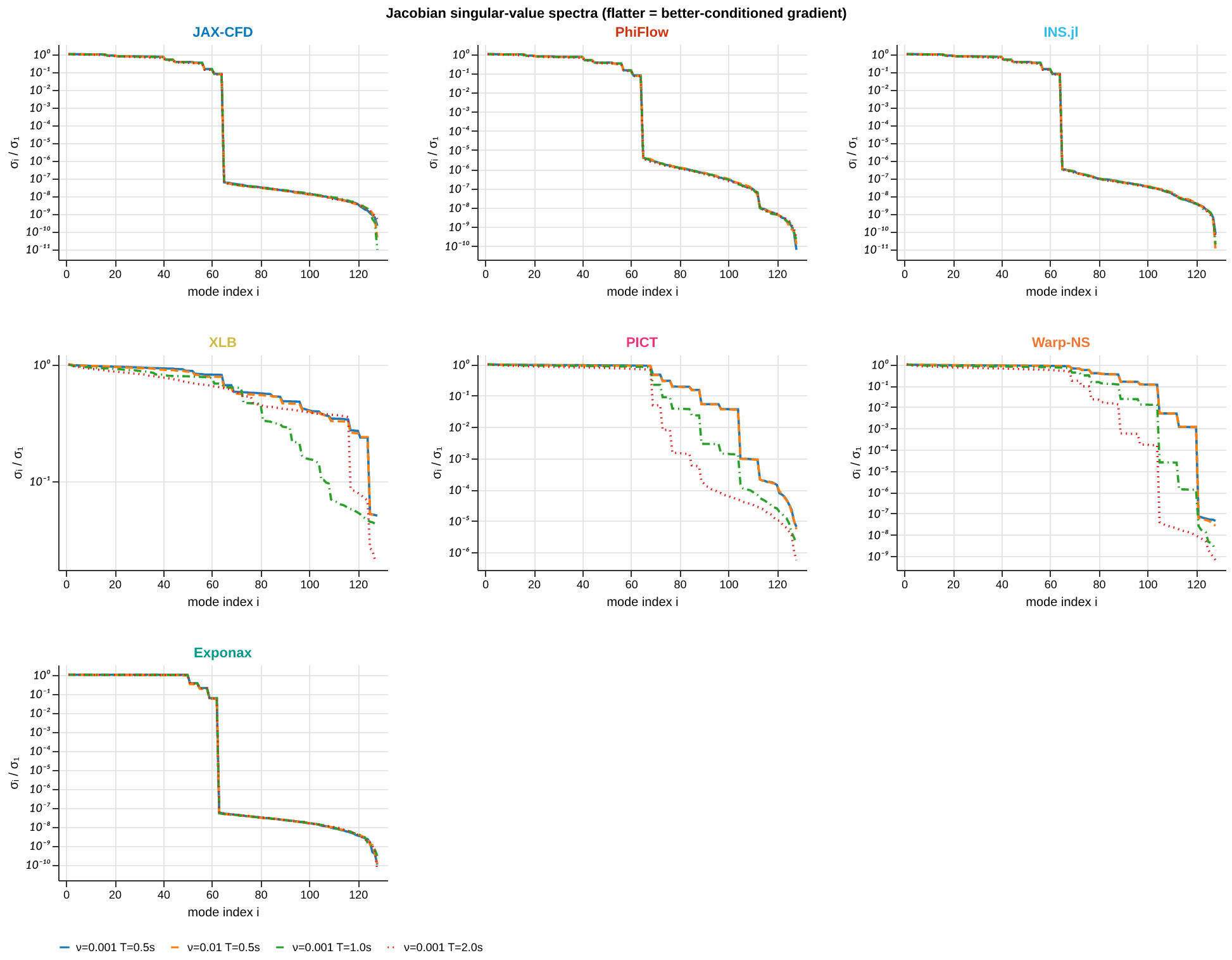
jacobian_svd

{
  "ic": {
    "name": "multimode",
    "seed": 42
  },
  "physics": {
    "N": 8,
    "nu": 0.001,
    "dt": 0.05,
    "steps": 10
  }
}

jacobian_svd_nu01

{
  "ic": {
    "name": "multimode",
    "seed": 42
  },
  "physics": {
    "N": 8,
    "nu": 0.01,
    "dt": 0.05,
    "steps": 10
  }
}

jacobian_svd_steps20

{
  "ic": {
    "name": "multimode",
    "seed": 42
  },
  "physics": {
    "N": 8,
    "nu": 0.001,
    "dt": 0.05,
    "steps": 20
  }
}

jacobian_svd_steps40

{
  "ic": {
    "name": "multimode",
    "seed": 42
  },
  "physics": {
    "N": 8,
    "nu": 0.001,
    "dt": 0.05,
    "steps": 40
  }
}

param_sweep

Sweeps nu ∈ {0.05, 0.01, 0.005, 0.001}

{
  "ic": {
    "name": "multimode",
    "seed": 42
  },
  "physics": {
    "N": 16,
    "dt": 0.05,
    "steps": 200,
    "nu": 0.05
  },
  "fd": {
    "eps_values": [
      5.0,
      1.0,
      0.1,
      0.01,
      0.001
    ],
    "n_dirs": 15
  },
  "sweep": {
    "key": "nu",
    "values": [
      0.05,
      0.01,
      0.005,
      0.001
    ]
  }
}

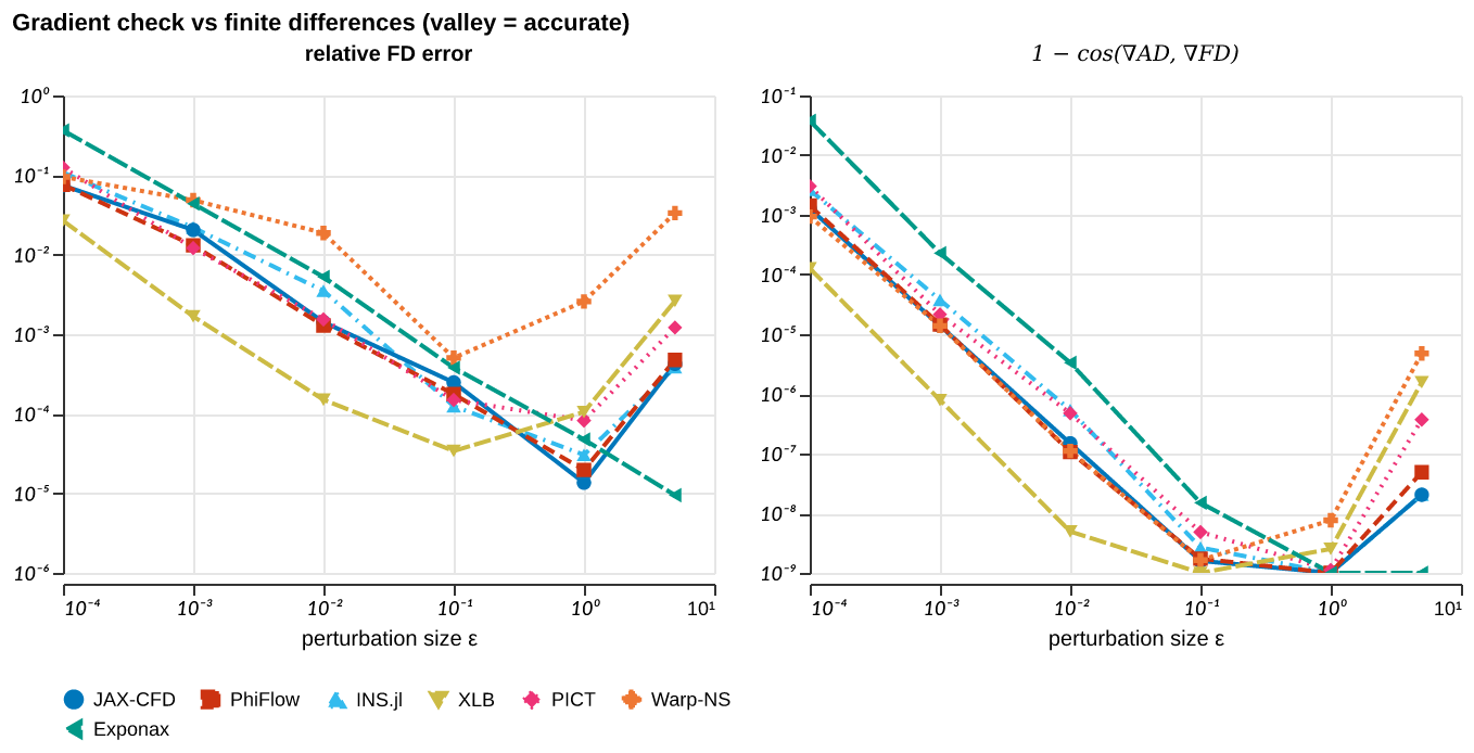
Gradient against finite differences

U-curves of finite-difference gradient error vs perturbation size \(\varepsilon\) together with subspace cosine; validates VJP correctness.

Settings

{
  "ic": {
    "name": "multimode",
    "seed": 42
  },
  "physics": {
    "N": 16,
    "nu": 0.001,
    "dt": 0.05,
    "steps": 20
  },
  "fd": {
    "eps_values": [
      5.0,
      1.0,
      0.1,
      0.01,
      0.001,
      0.0001
    ],
    "n_dirs": 20
  }
}

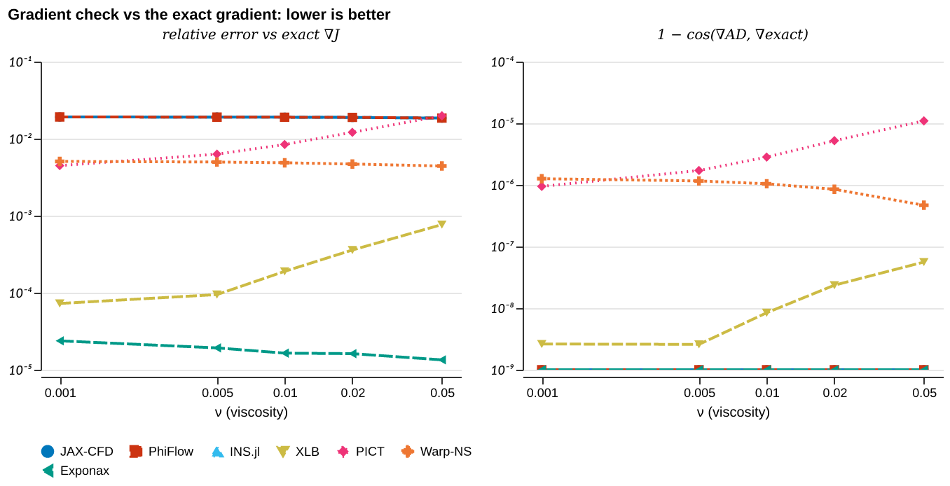
Gradient against the analytic Taylor–Green gradient

Relative error and 1 − cosine of each solver’s gradient of \(J = \sum \lvert\mathbf{u}(T)\rvert^2\) with respect to the TGV initial field, against the exact gradient \(\nabla J = 2 e^{-4\nu T}\,\mathbf{u}_0\). The closed form holds for divergence-free perturbations, so each gradient is compared after projecting out its curl-free part. There is no finite-difference step to tune, but the error includes the forward discretization error.

Settings

Sweeps nu ∈ {0.001, 0.005, 0.01, 0.02, 0.05}

{
  "ic": {
    "name": "tgv",
    "seed": 0
  },
  "physics": {
    "N": 32,
    "dt": 0.05,
    "steps": 20,
    "nu": 0.001
  },
  "reference": "<callable _tgv_analytic_grad>",
  "sweep": {
    "key": "nu",
    "values": [
      0.001,
      0.005,
      0.01,
      0.02,
      0.05
    ]
  },
  "project": "<callable project_divergence_free>"
}

Viscosity gradient against the analytic gradient

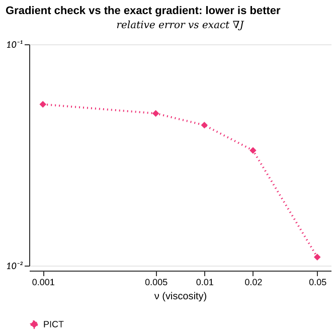
Relative error of each solver’s derivative of \(J = \sum \lvert\mathbf{u}(T)\rvert^2\) with respect to the viscosity for the TGV, against the exact \(dJ/d\nu = -4T\,J\) with \(J = e^{-4\nu T} \sum \lvert\mathbf{u}_0\rvert^2\) on the grid. The error includes the forward discretization error.

Settings

Sweeps nu ∈ {0.001, 0.005, 0.01, 0.02, 0.05}

{
  "ic": {
    "name": "tgv",
    "seed": 0
  },
  "physics": {
    "N": 32,
    "dt": 0.05,
    "steps": 20,
    "nu": 0.001
  },
  "reference": "<callable _tgv_analytic_dJ_dnu>",
  "sweep": {
    "key": "nu",
    "values": [
      0.001,
      0.005,
      0.01,
      0.02,
      0.05
    ]
  },
  "wrt": "viscosity"
}

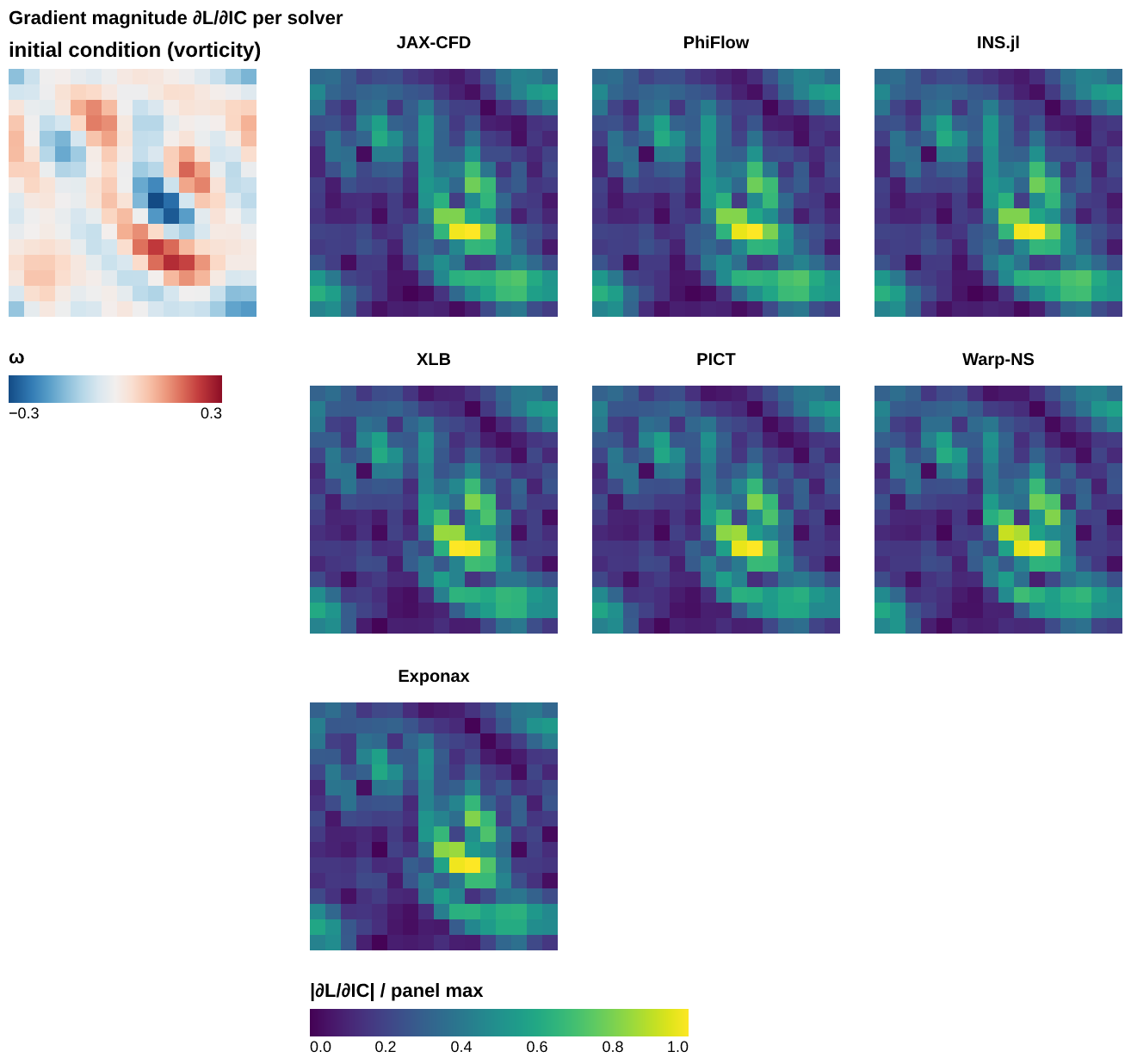
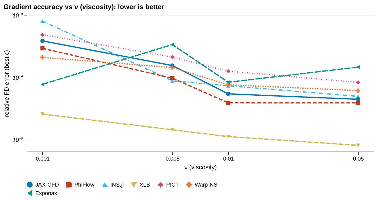
Gradient accuracy across the control parameter

Gradient norm, best-\(\varepsilon\) FD error, direction cosine, and U-curves vs the sweep parameter.

Settings

Sweeps nu ∈ {0.05, 0.01, 0.005, 0.001}

{
  "ic": {
    "name": "multimode",
    "seed": 42
  },
  "physics": {
    "N": 16,
    "dt": 0.05,
    "steps": 200,
    "nu": 0.05
  },
  "fd": {
    "eps_values": [
      5.0,
      1.0,
      0.1,
      0.01,
      0.001
    ],
    "n_dirs": 15
  },
  "sweep": {
    "key": "nu",
    "values": [
      0.05,
      0.01,
      0.005,
      0.001
    ]
  }
}

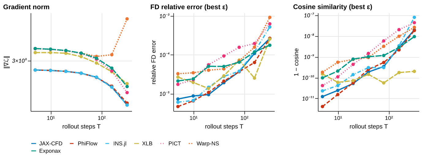
Gradient accuracy across rollout length

Gradient norm, FD error, and direction cosine vs rollout horizon \(T = \mathrm{steps}\cdot dt\).

Settings

Sweeps steps ∈ {5, 10, 20, 40, 80, 160, 320}

{
  "ic": {
    "name": "multimode",
    "seed": 42
  },
  "physics": {
    "N": 16,
    "nu": 0.001,
    "dt": 0.05,
    "steps": 5
  },
  "fd": {
    "eps_values": [
      1.0,
      0.1,
      0.01,
      0.001
    ],
    "n_dirs": 8
  },
  "sweep": {
    "key": "steps",
    "values": [
      5,
      10,
      20,
      40,
      80,
      160,
      320
    ]
  }
}

Results by solver

Solver	Best-ε FD error	1 − cosine
Exponax	4.06e-06	1.45e-11
jax-cfd	7.12e-06	3.51e-11
XLB	1.15e-05	1.67e-10
PhiFlow	1.26e-05	7.52e-11
INS.jl	1.58e-05	1.01e-10
Warp-NS	4.07e-05	1.64e-09
PICT	4.59e-05	1.12e-09

From Gradient against finite differences.