Forced Kolmogorov flow

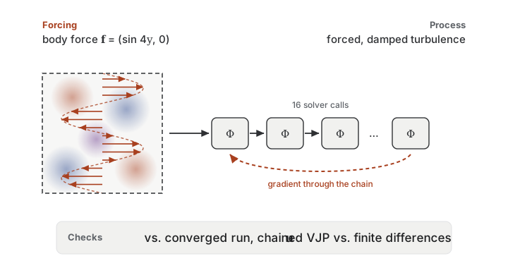
F2 Navier–Stokes (2D) Generated 2026-11-06 17:21 UTC 4 plots

Forced 2D turbulence that settles into a statistically steady state, and gradients through a chain of solver calls, as in training a model through a solver.

Incompressible fluid flow in 2D. We solve and differentiate through the 2D incompressible Navier–Stokes equations \(\partial_t \mathbf{u} + (\mathbf{u}\cdot\nabla)\mathbf{u} = -\nabla p + \nu\,\nabla^2\mathbf{u}\), \(\nabla\cdot\mathbf{u}=0\), with the kinematic viscosity \(\nu\) as the primary control parameter. The problem has three setups: a doubly periodic box, a channel flow past a cylinder, and a forced Kolmogorov flow.

The Kolmogorov flow adds a steady body force \(\mathbf{f} = (\sin 4y, 0)\) and a linear drag \(-\alpha\mathbf{u}\) to the right-hand side. The force drives the flow, and the drag removes the energy that piles up at the largest scales, so the turbulent flow settles into a statistically steady state.

How these results were produced

These are example results, produced automatically on GitHub-hosted runners and refreshed on every release. Each solver runs on its intended device: GPU-capable solvers on a Tesla T4 GPU node, CPU-only solvers (OpenFOAM, deal.II, FEniCS, Firedrake, TopOpt.jl) on a separate CPU node. Each benchmark job has its virtual machine to itself, but the hardware and the load on the host can change from run to run, so wall-clock times vary. Read them for relative scaling between solvers rather than as absolute timings. Accuracy and gradient metrics change little across hardware, although float32 arithmetic is not identical across devices and chaotic rollouts amplify small discrepancies. For numbers that reflect your setup, run the benchmark yourself on your target hardware.

Boundary conditions

Doubly periodic square domain \([0, 2\pi]^2\) (the flow wraps around at every edge), with incompressibility \(\nabla\cdot\mathbf{u}=0\) enforced by a pressure projection at each time step.

Checks

The results overview explains the columns and states.

Solver	Forward	Gradient	Cost to 10% error	Effort
GPU solversMultiples of the fastest GPU solver
PICT	Pass	Pass	16.2 sfastest	L0
Exponax	Not run	Not run	—	L3
INS.jl	Not run	Not run	—	L0
jax-cfd	Not run	Not run	—	L2
PhiFlow	Not run	Not run	—	L3
Warp-NS	Not run	Unstable	—	L2
XLB modified setup	Not run	Not run	—	L2
CPU solvers
OpenFOAM	Not implemented	Not supported	—	L0

Solvers differ in how general they are. Exponax and jax-cfd do not run Channel flow past a cylinder.

Modified setups (1)

These solvers run a substitute for part of the setup, so their checks hold for the modified setup.

XLB: Sub-steps each step to bound the Mach number. Effect: LBM ties the time step to the grid through the lattice Mach number, so XLB runs k times the prescribed number of steps (k = 9 at N = 256 on the 2-D box), and its cost includes them. Without sub-stepping the Taylor-Green case ran at Ma of about 0.88, with errors 84 to 114x the peer median.

Flags and exclusions (20)

Exponax on forward/kolmogorov: not run
Exponax on forward/kolmogorov_laminar: not run
Exponax on gradient/chain_fd_check: not run
INS.jl on forward/kolmogorov: not run
INS.jl on forward/kolmogorov_laminar: not run
INS.jl on gradient/chain_fd_check: not run
jax-cfd on forward/kolmogorov: not run
jax-cfd on forward/kolmogorov_laminar: not run
jax-cfd on gradient/chain_fd_check: not run
OpenFOAM on forward/kolmogorov: not implemented. this tesseract runs icoFoam, which has no momentum source term, so it cannot apply the body force or the drag. OpenFOAM's foamRun incompressibleFluid solver supports both through an fvModel, but this tesseract does not use it
OpenFOAM on forward/kolmogorov_laminar: not implemented. this tesseract runs icoFoam, which has no momentum source term, so it cannot apply the body force or the drag. OpenFOAM's foamRun incompressibleFluid solver supports both through an fvModel, but this tesseract does not use it
PhiFlow on forward/kolmogorov: not run
PhiFlow on forward/kolmogorov_laminar: not run
PhiFlow on gradient/chain_fd_check: not run
Warp-NS on forward/kolmogorov: not run
Warp-NS on forward/kolmogorov_laminar: not run
Warp-NS on gradient/chain_fd_check: unstable. the solver advances with explicit Euler and central differences for advection, which is linearly unstable at the timestep of the chain (see forward/kolmogorov). Over the chain's calls the unstable modes grow, so they dominate both the gradient and the finite differences, which then disagree at every ε a float32 run resolves. Where they grow fast enough, the chain from the ground-truth state diverges
XLB on forward/kolmogorov: not run
XLB on forward/kolmogorov_laminar: not run
XLB on gradient/chain_fd_check: not run

Not supported (1 solver)

OpenFOAM, 1 experiment. OpenFOAM is non-differentiable (C++, no AD path); DAFoam/OpenFOAM-AD exist but are not deployed in this tesseract

Forward

Is the prediction right? Forward experiments compare each solver’s output with a trusted reference, an analytic solution where one exists, and the other solvers.

Accuracy and speed on turbulent Kolmogorov flow

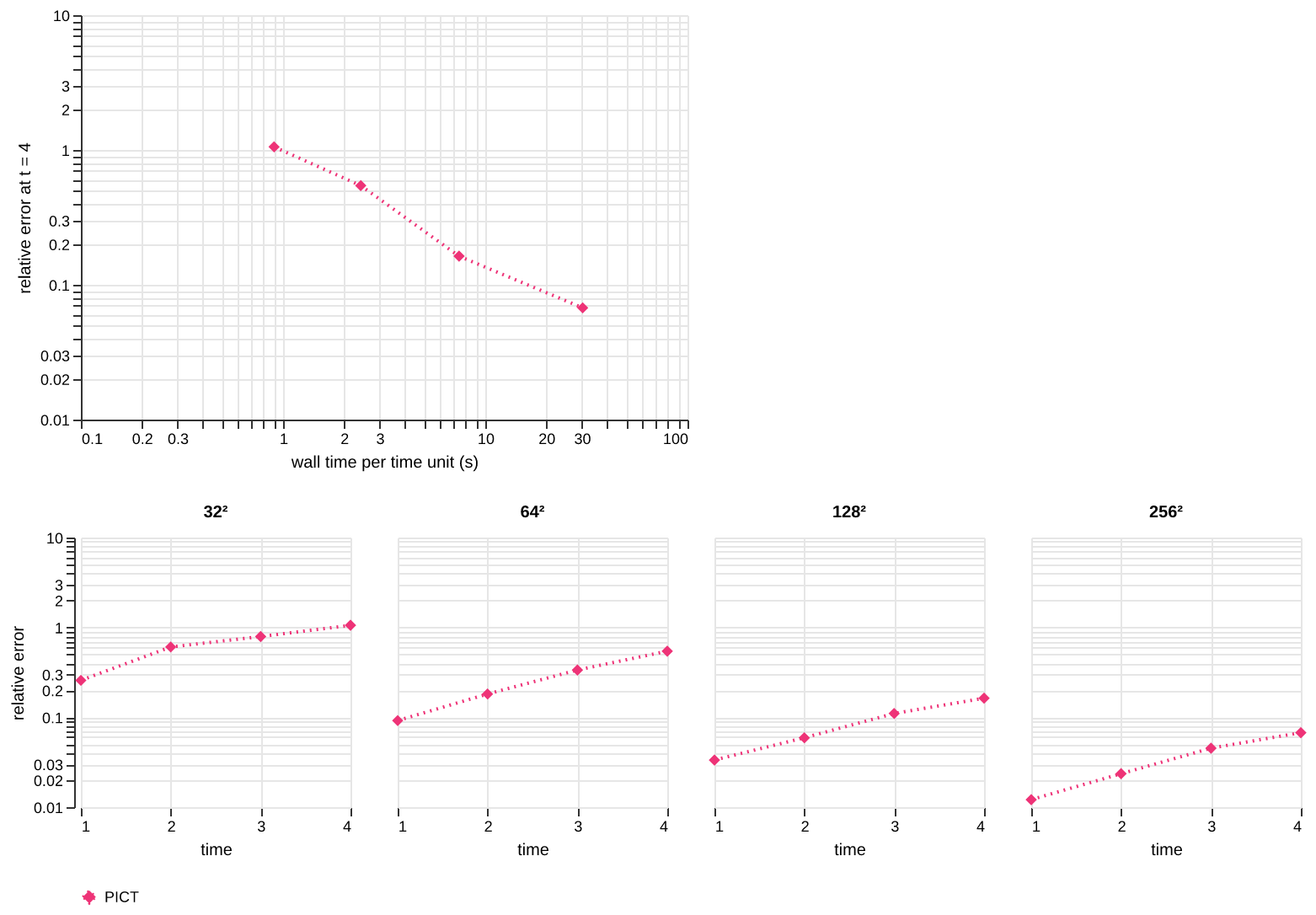
Each solver on 32² to 256² grids against a converged Exponax run at 1024², from three turbulent states of the Kolmogorov flow at ν = 2·10⁻³. Every grid runs at the CFL number of 64² with dt = 0.01 and is scored on the 64² grid. Relative error at t = 4 against the wall time of one time unit, and relative error per time on each grid, as medians over the states.

Settings

{
  "physics": {
    "N": 64,
    "dt": 0.01,
    "grids": [
      32,
      64,
      128,
      256
    ],
    "nu": 0.002,
    "forcing_wavenumber": 4,
    "forcing_amplitude": 1.0,
    "linear_drag": 0.1
  },
  "reference": "<callable generate_ground_truth>"
}

Accuracy on the laminar Kolmogorov transient

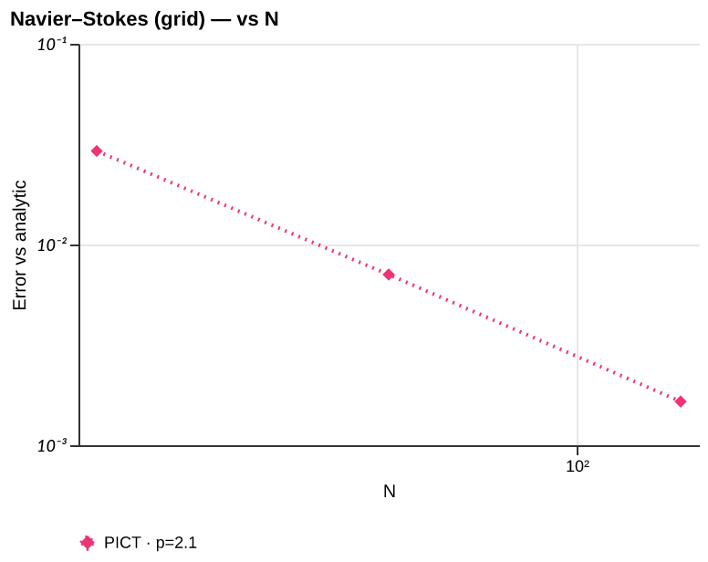
Relative error vs grid resolution \(N\) of the flow that the Kolmogorov force \((A\sin(\kappa y), 0)\), \(\kappa = 4\), drives from rest against linear drag, at \(t = 2\). The flow stays a shear flow, so it has the exact solution \(u = (A/\lambda)(1 - e^{-\lambda t}) \sin(\kappa y)\) with \(\lambda = \nu\kappa^2 + \alpha\). The timestep is small enough that the error is the spatial one.

Settings

Sweeps N ∈ {32, 64, 128}

{
  "ic": {
    "name": "rest",
    "seed": 0
  },
  "physics": {
    "N": 32,
    "nu": 0.05,
    "dt": 0.002,
    "steps": 1000,
    "forcing_wavenumber": 4,
    "forcing_amplitude": 1.0,
    "linear_drag": 0.1
  },
  "reference": "<callable laminar_reference>",
  "sweep": {
    "key": "N",
    "values": [
      32,
      64,
      128
    ]
  }
}

Gradient

Is the gradient right? Gradient experiments compare each solver’s AD or adjoint gradient with finite differences, in magnitude (relative \(L^2\) error) and direction (cosine similarity).

Gradient through chained solver calls

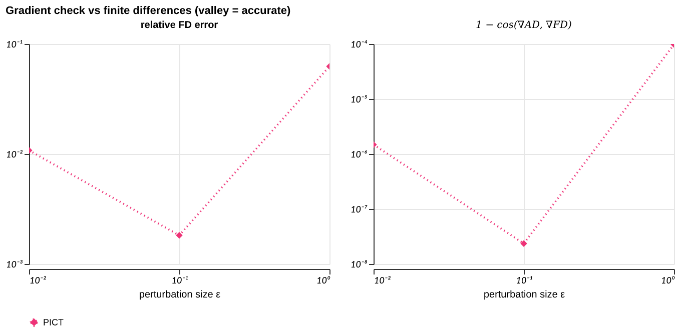
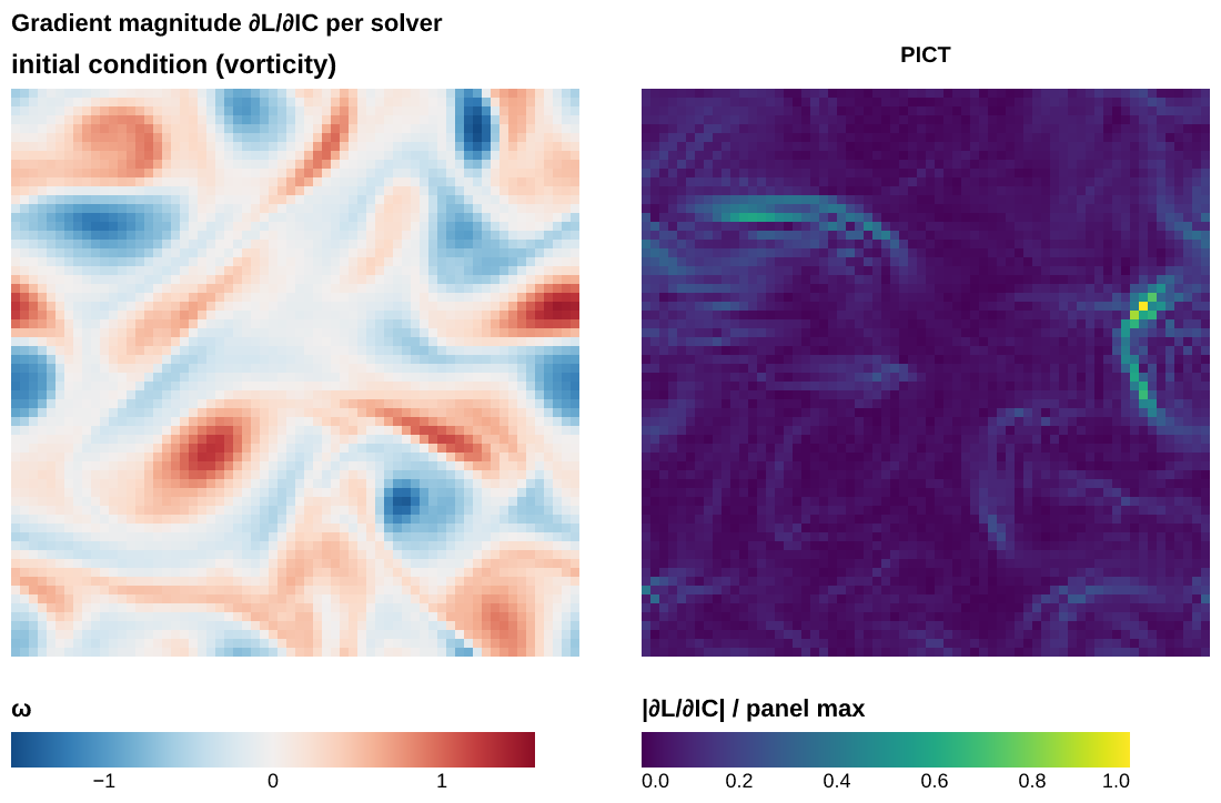
Finite-difference check of the gradient of a loss on 16 chained solver calls of 0.1 time units each, on the Kolmogorov flow at 64² and dt = 0.01, from a turbulent state of its ground truth plus a 1% divergence-free offset. The loss is the mean relative squared distance to the solver’s chain from that state, as in training through a solver, so its cotangents are far smaller than those of the single-call checks. Error and 1 − cos against ε, over 8 divergence-free directions.

Settings

{
  "physics": {
    "N": 64,
    "dt": 0.01,
    "steps": 10,
    "intervals": 16,
    "offset": 0.01,
    "nu": 0.002,
    "forcing_wavenumber": 4,
    "forcing_amplitude": 1.0,
    "linear_drag": 0.1
  },
  "fd": {
    "eps_values": [
      1.0,
      0.1,
      0.01
    ],
    "n_dirs": 8
  }
}