Learned Closure: Training a Neural Viscosity Model Through a PDE Solver (PyTorch)

In this tutorial, you will learn how to:

1. Build a Tesseract that wraps a single-timestep differentiable PDE solver (a 1D Burgers’ equation solver) and exposes a vector-Jacobian product.

2. Use Tesseract-Torch to call the served solver as a native PyTorch autograd layer via apply_tesseract, so gradients flow through the container automatically.

3. Train a neural network closure end-to-end through the containerized solver, differentiating through the entire time-stepping loop.

4. Compare the learned closure against baselines (a pure physics model and a pure ML model).

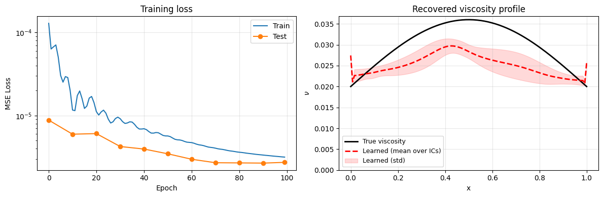
We will replace the viscosity model of a Burgers’ equation solver, normally a hand-tuned constant, with a small neural network, and train it so that it recovers the true (unknown) viscosity profile from solution data alone.

This is a small end-to-end example of embedding a learned closure into a solver with Tesseract. The closure is called once per solver step, which is the right structure when the physics genuinely needs a per-step update. It is deliberately kept simple so the moving parts are easy to follow; the What’s next section at the end points to the tricks real closures usually need.

Context

Closure modeling is a recurring problem across computational science: a simulation resolves the large scales but needs a model for the unresolved physics, such as a turbulence closure, a sub-grid scheme, or a constitutive law. These closures are often hand-tuned or empirical, and a natural idea is to learn them from data instead (Duraisamy, Iaccarino & Xiao, 2019). The catch is that a closure only makes sense inside the solver: to train it well, gradients have to flow from the simulation output, through the solver, and back into the network (Um et al., 2020; Shankar et al., 2023).

This is hard in practice because the solver is usually not a 30-line function you can import into your training script. It is often a heavyweight simulator with its own runtime, dependencies, and adjoint: a Fortran/C++ CFD code, a legacy in-house solver, or something differentiated by Enzyme at the LLVM IR level.

Tesseract is most useful for that hard case: a big, expensive simulator with a gnarly toolchain (a specific compiler, MPI, a licensed library, a non-Python runtime, a hand-written adjoint) that you want to hide behind a clean differentiable interface. The Burgers’ solver used here is the opposite: a few lines of NumPy/Torch, cheap to run, and trivially import-able, so on its own it needs no container at all and the HTTP round-trip dominates its runtime. We use it precisely because it is cheap, so the whole demo runs in a few minutes. The composition pattern below is identical either way; only the overhead changes.

With Tesseracts, we wrap the solver in a container that exposes a clean differentiable interface, and call it over HTTP as a single layer inside an otherwise ordinary PyTorch training loop. The neural network lives in native PyTorch; the solver lives in a Docker image. Tesseract-Torch registers the served solver as a PyTorch autograd custom function, so loss.backward() dispatches a vector-Jacobian product (VJP) call back through the solver automatically, the analogue of what Tesseract-JAX does for JAX in the other demos in this series.

The components

• burgers_solver (containerized Tesseract): a single-timestep Burgers’ equation solver. Takes the current velocity field u and a viscosity field nu, returns the velocity field after one explicit Euler step, a pure physics component with the interface \((u, \nu, dt) \to u_\text{next}\). It exposes a VJP, so it slots into PyTorch autograd like any other layer, even though it runs in a separate container.

• ViscosityNet (torch.nn.Module): a small MLP that maps local flow features \((u, \partial u/\partial x, x)\) to a viscosity field \(\nu\). An ordinary network, trained with a standard optimizer, in this process.

At each timestep the outer loop calls the network directly to predict \(\nu\), then calls the solver via apply_tesseract to advance one step (shown in full in Step 4).

To learn more about building and running Tesseracts, please refer to the Tesseract documentation.

import os

import matplotlib.pyplot as plt
import numpy as np
import torch
import torch.nn as nn
from tesseract_torch import apply_tesseract

from tesseract_core import Tesseract

torch.set_default_dtype(torch.float64)

# Workload size. Every solver call is an HTTP round-trip to the container, so
# the defaults are modest to keep the demo (and CI) to a few minutes.
# Set FULL_RUN=1 for the publication-quality run used to produce the figures.
FULL_RUN = os.environ.get("FULL_RUN", "0") == "1"

# Time step. The spatially-varying viscosity only becomes identifiable once
# diffusion has acted appreciably over the rollout, so we use a dt large enough
# for the closure to actually "feel" the viscosity profile (well within the
# explicit-diffusion CFL limit nu*dt/dx^2 < 0.5; here nu_max*dt/dx^2 ≈ 0.40).
# Too small a dt and every viscosity profile fits the data equally well: the
# closure can't recover the shape no matter how long it trains. Using a larger
# dt also lets us keep the rollout short. The closure is called once per step
# and we backprop through the whole chain, so fewer steps means a cheaper,
# better-behaved gradient. A real, longer rollout would reach for gradient
# checkpointing here (see the "What's next" section).
DT = 5e-4
LR = 5e-3

if FULL_RUN:
    N_TRAIN, N_TEST = 8, 4
    N_STEPS = 40
    N_EPOCHS = 300
    DIRECT_EPOCHS = 300
else:
    # Small but enough to recover the viscosity hump and beat the constant
    # baseline.
    N_TRAIN, N_TEST = 3, 2
    N_STEPS = 20
    N_EPOCHS = 100
    DIRECT_EPOCHS = 100

print(
    f"FULL_RUN={FULL_RUN}: {N_TRAIN} train / {N_TEST} test ICs, "
    f"{N_STEPS} steps, {N_EPOCHS} epochs, dt={DT}"
)

# Grid setup (must match the solver)
N = 128
DX = 1.0 / (N - 1)
X = torch.linspace(0.0, 1.0, N)

FULL_RUN=False: 3 train / 2 test ICs, 20 steps, 100 epochs, dt=0.0005

Step 1: Build and serve the solver Tesseract

We build the solver into a Docker image with tesseract build, then serve it in a container and call it over HTTP, the same way you would deploy a real simulator. The training loop below never imports the solver’s code; it only ever talks to the running container.

First, build the image (this can take a few minutes the first time):

%%bash
tesseract build burgers_solver/

 [i] Building image ...
⠋ Processing
 [i] Built image sha256:270b9738ccf8, ['burgers-solver:0.1.0', 'burgers-solver:latest']

["burgers-solver:0.1.0", "burgers-solver:latest"]

Now load the built image and start a server container. serve() launches the container; we tear it down at the end of the notebook to free resources.

solver_tess = Tesseract.from_image("burgers-solver")
solver_tess.serve()
print(f"Solver endpoints: {solver_tess.available_endpoints}")

Solver endpoints: ['apply', 'jacobian', 'jacobian_vector_product', 'vector_jacobian_product', 'health', 'abstract_eval', 'test']

Step 2: The ground truth — Burgers’ equation with spatially-varying viscosity

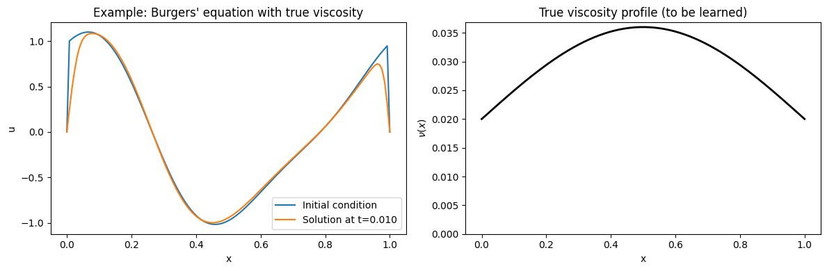
We generate training data from a Burgers’ equation with a known but non-trivial viscosity profile:

\[\nu_{\text{true}}(x) = \nu_0 \left(1 + A \sin(\pi x)\right)\]

This represents a spatially-varying material property, analogous to a turbulence closure, constitutive law, or sub-grid model that varies across the domain. The neural closure’s job is to recover this profile from solution data alone.

The reference solutions come from the same served solver, called forward-only (no gradients); there is no second copy of the physics anywhere in this notebook.

# True viscosity profile
NU_0 = 0.02
A = 0.8
nu_true = NU_0 * (1.0 + A * torch.sin(np.pi * X))


def burgers_reference(u0, nu_field, dt, n_steps):
    """Reference solution with a prescribed viscosity field (no neural network).

    Calls the served solver Tesseract forward-only via `.apply()`. This is just
    data generation, so it stays outside autograd. `.apply()` returns decoded
    NumPy arrays, which we wrap back into tensors.
    """
    u = u0.clone()
    for _ in range(n_steps):
        out = solver_tess.apply({"u": u, "nu": nu_field, "dt": dt})
        # .apply() returns a (possibly read-only) NumPy array decoded from JSON;
        # copy into a fresh tensor so PyTorch is happy.
        u = torch.tensor(np.asarray(out["u_next"]))
    return u


def make_ic(seed):
    """Random smooth initial condition: sum of low-frequency sinusoids."""
    rng = torch.Generator().manual_seed(seed)
    a1 = 0.5 + 0.5 * torch.rand(1, generator=rng).item()
    a2 = 0.3 * torch.rand(1, generator=rng).item()
    phase = torch.rand(1, generator=rng).item() * np.pi
    u0 = a1 * torch.sin(2 * np.pi * X + phase) + a2 * torch.sin(4 * np.pi * X)
    u0[0] = 0.0
    u0[-1] = 0.0
    return u0


train_ics = torch.stack([make_ic(i) for i in range(N_TRAIN)])
test_ics = torch.stack([make_ic(N_TRAIN + i) for i in range(N_TEST)])

with torch.no_grad():
    train_targets = torch.stack(
        [burgers_reference(ic, nu_true, DT, N_STEPS) for ic in train_ics]
    )
    test_targets = torch.stack(
        [burgers_reference(ic, nu_true, DT, N_STEPS) for ic in test_ics]
    )

print(f"Training set: {N_TRAIN} initial conditions -> solutions")
print(f"Test set:     {N_TEST} initial conditions -> solutions")
print(f"Grid: {N} points, dt={DT}, {N_STEPS} steps")

# Visualize one example
fig, axes = plt.subplots(1, 2, figsize=(12, 4))
axes[0].plot(X.numpy(), train_ics[0].numpy(), label="Initial condition")
axes[0].plot(
    X.numpy(), train_targets[0].numpy(), label=f"Solution at t={DT * N_STEPS:.3f}"
)
axes[0].set_xlabel("x")
axes[0].set_ylabel("u")
axes[0].legend()
axes[0].set_title("Example: Burgers' equation with true viscosity")

axes[1].plot(X.numpy(), nu_true.numpy(), "k-", linewidth=2)
axes[1].set_xlabel("x")
axes[1].set_ylabel(r"$\nu(x)$")
axes[1].set_title("True viscosity profile (to be learned)")
axes[1].set_ylim(bottom=0)

plt.tight_layout()
plt.show()

Training set: 3 initial conditions -> solutions
Test set:     2 initial conditions -> solutions
Grid: 128 points, dt=0.0005, 20 steps

Step 3: The neural closure — a plain PyTorch module

The closure is an ordinary torch.nn.Module: a small MLP with 2 hidden layers of 32 units. It maps the local flow features \((u, \partial u/\partial x, x)\) at each grid point to a viscosity value. There is nothing Tesseract-specific about it; it is the network the closure researcher brings, trained with a standard optimizer, entirely in this process.

A sigmoid keeps the predicted viscosity in a physically reasonable range \([0, \nu_{\max}]\), which also prevents CFL violations in the explicit solver.

class ViscosityNet(nn.Module):
    """MLP closure: local flow features (u, du/dx, x) -> viscosity nu."""

    def __init__(self, hidden_dim=32, nu_max=0.05):
        super().__init__()
        self.nu_max = nu_max
        self.net = nn.Sequential(
            nn.Linear(3, hidden_dim),
            nn.Tanh(),
            nn.Linear(hidden_dim, hidden_dim),
            nn.Tanh(),
            nn.Linear(hidden_dim, 1),
        )

    def forward(self, u, dudx, x):
        features = torch.stack([u, dudx, x], dim=-1)  # (N, 3)
        out = self.net(features)[:, 0]  # (N,)
        return self.nu_max * torch.sigmoid(out)


torch.manual_seed(1)
closure = ViscosityNet()
n_params = sum(p.numel() for p in closure.parameters())
print(f"Closure parameters: {n_params}")

# Sanity check: the untrained closure produces sensible viscosities
with torch.no_grad():
    dudx0 = torch.gradient(train_ics[0], spacing=(DX,))[0]
    nu0 = closure(train_ics[0], dudx0, X)
print(f"Initial viscosity range: [{float(nu0.min()):.4f}, {float(nu0.max()):.4f}]")

Closure parameters: 1217
Initial viscosity range: [0.0204, 0.0310]

Step 4: End-to-end training through the containerized solver

The training loss is:

\[\mathcal{L}(\theta) = \frac{1}{M} \sum_{i=1}^{M} \left\| u_{\text{solver}}(u_0^{(i)}; \nu_\theta) - u_{\text{data}}^{(i)} \right\|^2\]

where \(\nu_\theta\) is the neural viscosity closure with parameters \(\theta\), and \(u_{\text{solver}}\) runs the full Burgers’ equation with \(\nu_\theta\) called at every timestep.

The time-stepping loop calls the network directly and the solver via apply_tesseract:

for each timestep:
    nu = closure(u, dudx, x)                              # plain torch
    u  = apply_tesseract(solver, {u, nu, dt})["u_next"]   # HTTP call to container

loss.backward() differentiates through the entire loop: through every timestep, through a VJP HTTP request to the container at each step, and into the network weights, all automatically.

def solve_with_closure(u0, closure, dt, n_steps):
    """Run the full time-stepping loop, calling the served solver each step.

    The closure is plain in-process PyTorch; the solver is the containerized
    differentiable layer, reached over HTTP. In production this same loop would
    drive a Fortran solver with an adjoint, with only the served image changing.
    """
    u = u0
    for _step in range(n_steps):
        dudx = torch.zeros_like(u)
        dudx[1:-1] = (u[2:] - u[:-2]) / (2 * DX)

        nu = closure(u, dudx, X)  # closure: predict viscosity (native torch)

        # Solver: one explicit Euler step, executed in the container
        solver_out = apply_tesseract(solver_tess, {"u": u, "nu": nu, "dt": dt})
        u = solver_out["u_next"]
    return u


def loss_batch(closure, ics, targets):
    """Mean MSE over a batch of initial conditions."""
    preds = torch.stack(
        [solve_with_closure(ics[i], closure, DT, N_STEPS) for i in range(ics.shape[0])]
    )
    return torch.mean((preds - targets) ** 2)


# Verify the forward pass + gradient flow
print("Testing forward pass + gradient...")
l0 = loss_batch(closure, train_ics, train_targets)
l0.backward()
grad_norm = torch.sqrt(
    sum(p.grad.pow(2).sum() for p in closure.parameters() if p.grad is not None)
)
print(f"  Initial loss: {float(l0.detach()):.6e}")
print(f"  Gradient norm: {float(grad_norm):.6e}")
print("  Gradients flow: loss -> solver VJP (HTTP) -> network weights.")
closure.zero_grad()

Testing forward pass + gradient...
  Initial loss: 1.283973e-04
  Gradient norm: 1.046508e-03
  Gradients flow: loss -> solver VJP (HTTP) -> network weights.

Gradient validation against finite differences

Correctness check: the AD gradient (loss → solver VJP over HTTP → network) matches finite differences to high precision.

# Finite difference check on a single weight element of the first layer.
ics_sub = train_ics[:2]
tgt_sub = train_targets[:2]

# AD gradient
closure.zero_grad()
loss_val = loss_batch(closure, ics_sub, tgt_sub)
loss_val.backward()

w = closure.net[0].weight.data  # first Linear layer (raw tensor, no autograd)
idx = (0, 0)
ad = float(closure.net[0].weight.grad[idx])

# Finite difference
eps = 1e-5
orig = w[idx].item()
with torch.no_grad():
    w[idx] = orig + eps
    l_plus = float(loss_batch(closure, ics_sub, tgt_sub))
    w[idx] = orig - eps
    l_minus = float(loss_batch(closure, ics_sub, tgt_sub))
    w[idx] = orig  # restore

fd = (l_plus - l_minus) / (2 * eps)
rel_err = abs(ad - fd) / (abs(fd) + 1e-30)
print(f"{'AD':>14s} {'FD':>14s} {'Rel. Error':>12s}")
print(f"{ad:14.6e} {fd:14.6e} {rel_err:12.2e}")
closure.zero_grad()

            AD             FD   Rel. Error
 -6.627976e-07  -6.627976e-07     6.68e-10

Training loop

# Re-initialize for a clean training run
torch.manual_seed(1)
closure = ViscosityNet()
optimizer = torch.optim.Adam(closure.parameters(), lr=LR)

train_losses = []
test_losses = []

print("Training neural closure through the solver...")
for epoch in range(N_EPOCHS):
    optimizer.zero_grad()
    train_loss = loss_batch(closure, train_ics, train_targets)
    train_loss.backward()
    optimizer.step()
    train_losses.append(float(train_loss.detach()))

    if epoch % 10 == 0 or epoch == N_EPOCHS - 1:
        with torch.no_grad():
            test_loss = float(loss_batch(closure, test_ics, test_targets))
        test_losses.append((epoch, test_loss))
        print(
            f"  Epoch {epoch:4d}: train loss = {train_losses[-1]:.4e}, "
            f"test loss = {test_loss:.4e}"
        )

print(f"\nFinal train loss: {train_losses[-1]:.4e}")
print(f"Final test loss:  {test_losses[-1][1]:.4e}")

Training neural closure through the solver...
  Epoch    0: train loss = 1.2840e-04, test loss = 8.8252e-06
  Epoch   10: train loss = 1.1664e-05, test loss = 5.9784e-06
  Epoch   20: train loss = 1.1159e-05, test loss = 6.0776e-06
  Epoch   30: train loss = 9.1783e-06, test loss = 4.2518e-06
  Epoch   40: train loss = 6.9523e-06, test loss = 3.9642e-06
  Epoch   50: train loss = 5.6923e-06, test loss = 3.4751e-06
  Epoch   60: train loss = 4.7374e-06, test loss = 2.9877e-06
  Epoch   70: train loss = 4.0577e-06, test loss = 2.7151e-06
  Epoch   80: train loss = 3.6290e-06, test loss = 2.7027e-06
  Epoch   90: train loss = 3.3559e-06, test loss = 2.6873e-06
  Epoch   99: train loss = 3.1723e-06, test loss = 2.7432e-06

Final train loss: 3.1723e-06
Final test loss:  2.7432e-06

fig, axes = plt.subplots(1, 2, figsize=(12, 4))

axes[0].semilogy(train_losses, label="Train")
test_epochs, test_vals = zip(*test_losses, strict=False)
axes[0].semilogy(test_epochs, test_vals, "o-", label="Test")
axes[0].set_xlabel("Epoch")
axes[0].set_ylabel("MSE Loss")
axes[0].set_title("Training loss")
axes[0].legend()
axes[0].grid(True, alpha=0.3)

# Compare learned viscosity to true viscosity, averaged over training ICs.
nu_samples = []
with torch.no_grad():
    for ic in train_ics:
        dudx = torch.zeros_like(ic)
        dudx[1:-1] = (ic[2:] - ic[:-2]) / (2 * DX)
        nu_samples.append(closure(ic, dudx, X))
nu_samples = torch.stack(nu_samples)
nu_mean = nu_samples.mean(dim=0)
nu_std = nu_samples.std(dim=0)

x_np = X.numpy()
axes[1].plot(x_np, nu_true.numpy(), "k-", linewidth=2, label="True viscosity")
axes[1].plot(x_np, nu_mean.numpy(), "r--", linewidth=2, label="Learned (mean over ICs)")
axes[1].fill_between(
    x_np,
    (nu_mean - nu_std).numpy(),
    (nu_mean + nu_std).numpy(),
    color="r",
    alpha=0.15,
    label="Learned (std)",
)
axes[1].set_xlabel("x")
axes[1].set_ylabel(r"$\nu$")
axes[1].set_title("Recovered viscosity profile")
axes[1].legend(fontsize=9)
axes[1].set_ylim(bottom=0)
axes[1].grid(True, alpha=0.3)

plt.tight_layout()
plt.show()

Step 5: Baselines

We compare three approaches:

Model	Description
Constant viscosity	Burgers’ solver with \(\nu = \nu_0\) (the standard “wrong” closure)
Direct ML	MLP trained to map \(u_0 \to u_\text{final}\) directly, no physics
Learned closure	Neural \(\nu(u, \partial u/\partial x, x)\) trained through the solver (this demo)

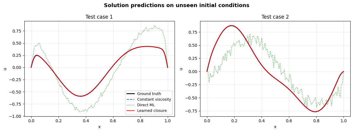
The closure here is not trained to convergence: the CI defaults keep the run to a few minutes, so the recovered viscosity profile is approximate. As a result the learned closure decisively beats the pure-ML baseline but only edges out the constant-viscosity baseline, which stays competitive at this short budget. Set FULL_RUN=1 for the longer run that sharpens the profile and widens that gap. The point of this demo is the composition pattern, not a state-of-the-art closure.

# --- Baseline 1: Constant (wrong) viscosity ---
nu_const = NU_0 * torch.ones(N)
with torch.no_grad():
    const_preds_test = torch.stack(
        [burgers_reference(ic, nu_const, DT, N_STEPS) for ic in test_ics]
    )
const_mse = float(torch.mean((const_preds_test - test_targets) ** 2))
print(f"Constant viscosity test MSE: {const_mse:.4e}")


# --- Baseline 2: Direct ML (MLP mapping u0 -> u_final, no physics) ---
class DirectNet(nn.Module):
    """Pure ML: maps the whole field u0 directly to u_final."""

    def __init__(self, n=N, hidden=128):
        super().__init__()
        self.net = nn.Sequential(
            nn.Linear(n, hidden),
            nn.Tanh(),
            nn.Linear(hidden, hidden),
            nn.Tanh(),
            nn.Linear(hidden, 64),
            nn.Tanh(),
            nn.Linear(64, n),
        )

    def forward(self, u0):
        return self.net(u0)


def direct_loss(model, ics, targets):
    preds = model(ics)
    return torch.mean((preds - targets) ** 2)


torch.manual_seed(2)
direct = DirectNet()
direct_opt = torch.optim.Adam(direct.parameters(), lr=1e-3)

print("\nTraining direct ML baseline...")
for epoch in range(DIRECT_EPOCHS):
    direct_opt.zero_grad()
    dl = direct_loss(direct, train_ics, train_targets)
    dl.backward()
    direct_opt.step()
    if epoch % 20 == 0:
        with torch.no_grad():
            test_dl = float(direct_loss(direct, test_ics, test_targets))
        print(
            f"  Epoch {epoch:4d}: train = {float(dl.detach()):.4e}, test = {test_dl:.4e}"
        )

with torch.no_grad():
    direct_test_mse = float(direct_loss(direct, test_ics, test_targets))
print(f"\nDirect ML test MSE: {direct_test_mse:.4e}")

# --- Learned closure (already trained above) ---
with torch.no_grad():
    learned_test_mse = float(loss_batch(closure, test_ics, test_targets))
print(f"Learned closure test MSE: {learned_test_mse:.4e}")

print(f"\n{'Model':<25s} {'Test MSE':>12s}")
print("-" * 40)
print(f"{'Constant viscosity':<25s} {const_mse:12.4e}")
print(f"{'Direct ML':<25s} {direct_test_mse:12.4e}")
print(f"{'Learned closure':<25s} {learned_test_mse:12.4e}")

Constant viscosity test MSE: 6.1354e-06

Training direct ML baseline...
  Epoch    0: train = 3.3670e-01, test = 2.0239e-01
  Epoch   20: train = 3.7105e-02, test = 1.1341e-01
  Epoch   40: train = 4.0102e-03, test = 7.2236e-02
  Epoch   60: train = 1.2106e-03, test = 7.4998e-02
  Epoch   80: train = 6.3123e-04, test = 7.7559e-02

Direct ML test MSE: 7.8228e-02
Learned closure test MSE: 2.7432e-06

Model                         Test MSE
----------------------------------------
Constant viscosity          6.1354e-06
Direct ML                   7.8228e-02
Learned closure             2.7432e-06

Step 6: Solution comparison on test data

For unseen initial conditions, we compare the three models’ predictions against the ground truth.

n_show = min(4, N_TEST)
ncols = 2 if n_show > 1 else 1
nrows = (n_show + ncols - 1) // ncols
fig, axes = plt.subplots(nrows, ncols, figsize=(6 * ncols, 4.5 * nrows), squeeze=False)

with torch.no_grad():
    direct_preds = direct(test_ics)
    for idx in range(n_show):
        ax = axes[idx // ncols][idx % ncols]
        ic = test_ics[idx]
        target = test_targets[idx]

        const_pred = burgers_reference(ic, nu_const, DT, N_STEPS)
        direct_pred = direct_preds[idx]
        learned_pred = solve_with_closure(ic, closure, DT, N_STEPS)

        ax.plot(x_np, target.numpy(), "k-", linewidth=2, label="Ground truth")
        ax.plot(
            x_np,
            const_pred.numpy(),
            "b--",
            linewidth=1.5,
            alpha=0.7,
            label="Constant viscosity",
        )
        ax.plot(
            x_np, direct_pred.numpy(), "g:", linewidth=1.5, alpha=0.7, label="Direct ML"
        )
        ax.plot(
            x_np, learned_pred.numpy(), "r-", linewidth=1.5, label="Learned closure"
        )
        ax.set_xlabel("x")
        ax.set_ylabel("u")
        ax.set_title(f"Test case {idx + 1}")
        ax.grid(True, alpha=0.3)
        if idx == 0:
            ax.legend(fontsize=9)

plt.suptitle(
    "Solution predictions on unseen initial conditions", fontsize=13, fontweight="bold"
)
plt.tight_layout()
plt.show()

Tear down the solver

Stop the solver container to free resources.

# Tear down Tesseract after use to prevent resource leaks
solver_tess.teardown()

Takeaways

In this tutorial, we trained a neural viscosity closure end-to-end through a containerized Burgers’ equation solver. Here are the key points:

1. Containerized solver, native ML. The solver runs in a Docker container served as a Tesseract; the closure is a plain in-process torch.nn.Module. The two compose in an outer time-stepping loop, with apply_tesseract bridging the container boundary at each step.

2. End-to-end gradients through the container. Because Tesseract-Torch registers the served solver as a PyTorch autograd function, loss.backward() dispatches the solver’s VJP over HTTP and flows the gradient into the network, with no hand-coded plumbing. We validated these gradients against finite differences.

3. Physics structure helps. Even with the short CI training budget, the learned closure beats the pure-ML baseline by orders of magnitude and edges out the constant-viscosity baseline, recovering the shape of the true viscosity profile from solution data alone. Training longer with FULL_RUN=1 widens the margin over the constant baseline.

4. Composability across a container boundary. The closure (plain torch) and the solver (a different image exposing the same \((u, \nu, dt) \to u_\text{next}\) contract) can be swapped independently. The training loop is identical regardless of what language the solver is written in or how its adjoint is produced.

5. Mind the overhead. Every solver call here is an HTTP round-trip, and a single explicit Euler step is cheap, so this demo is overhead-bound. Tesseract pays off when the solver step is expensive relative to the round-trip (a real CFD/FEM step, a remote or cross-language solver), or when you can space closure updates out over several steps. See the performance guide for the overhead breakdown and rules of thumb.

What’s next

This demo is the basic recipe. Real-world closures usually need more than a vanilla MLP trained with Adam through a single-step solver. Here are the directions to explore from here:

• Wrap a legacy solver. Replace the Burgers’ Tesseract with a Fortran/C++ solver that exposes an adjoint (for example via Enzyme). The closure training loop above works unchanged; only the image name changes.

• Train smarter. For small closures with a least-squares loss, a Gauss–Newton or L-BFGS solve on the point-wise residual Jacobian (forward-mode AD) can converge far faster than Adam and more readily unlearn spurious feature dependence.

• Get more data for free. Chain the solver to emit several snapshots per simulation and train on all of them: extra supervision at no extra simulation cost, and a natural reason to chunk the rollout into shorter segments.

• Go to longer rollouts. When the closure is called over many steps, use gradient checkpointing to keep memory bounded, and batch/vmap solver calls to amortize HTTP overhead (batching multiple initial conditions per request).

• Tackle a real closure. Swap the Burgers’ equation for a turbulence model, a climate sub-grid scheme, or a materials constitutive law.

• Explore other demos. See the CFD optimization, FEM shape optimization, and data assimilation demos for the JAX side of the same composition pattern.

Built something with these? We’d love to see it. Share your closure on the Tesseract Community Forum, and tell us where Tesseract’s overhead or UX got in your way so we can improve it.