Navier–Stokes (3D)
Auto-generated 2026-06-25 08:54 UTC · 9 plots
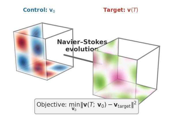
Recover the initial velocity field of a 3D turbulent flow from a later snapshot, differentiating through the Navier–Stokes rollout.
Fluid flow in 3D. The 3D counterpart of the 2D fluid problem, and the harder stress test for differentiable simulation: real turbulence lives in 3D, and the gradients are correspondingly more delicate.
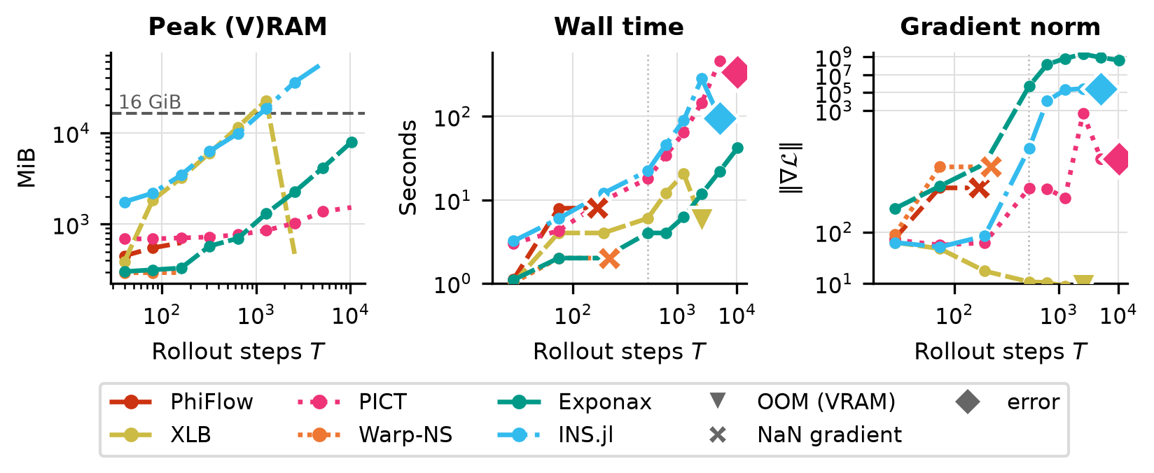
We solve the 3D incompressible Navier–Stokes equations \(\partial_t \mathbf{u} + (\mathbf{u}\cdot\nabla)\mathbf{u} = -\nabla p + \nu\,\nabla^2\mathbf{u}\), \(\nabla\cdot\mathbf{u}=0\), with viscosity \(\nu\) as the primary control parameter. Unlike 2D, the 3D equations admit vortex stretching, which amplifies vorticity and brings on chaos far sooner: the chaos horizon is \(T^\ast \approx 8\text{–}16\) s versus \(T^\ast > 64\) s in 2D (at \(\nu=10^{-3}\), \(N=16\)). As a result gradient norms grow along the rollout here rather than decaying as they do in 2D.
These are example results, produced automatically on GitHub Actions runners and refreshed on every release. Each solver runs on its intended device: GPU-capable solvers on a Tesla T4 GPU node, CPU-only solvers (OpenFOAM, deal.II, FEniCS, Firedrake) on a CPU node. Accuracy and gradient metrics are hardware-independent and reproducible. Wall-clock numbers reflect commodity cloud hardware and can vary by 10–15% between runs, so read them for relative scaling between solvers rather than as absolute timings. For numbers that reflect your setup, run the benchmarks yourself on your target hardware.
Triply-periodic cubic domain \([0, 2\pi]^3\) (the flow wraps around on all three axes). Incompressibility \(\nabla\cdot\mathbf{u}=0\) is enforced by a pressure projection at each time step. No walls or inflow/outflow boundaries.
Initial Conditions
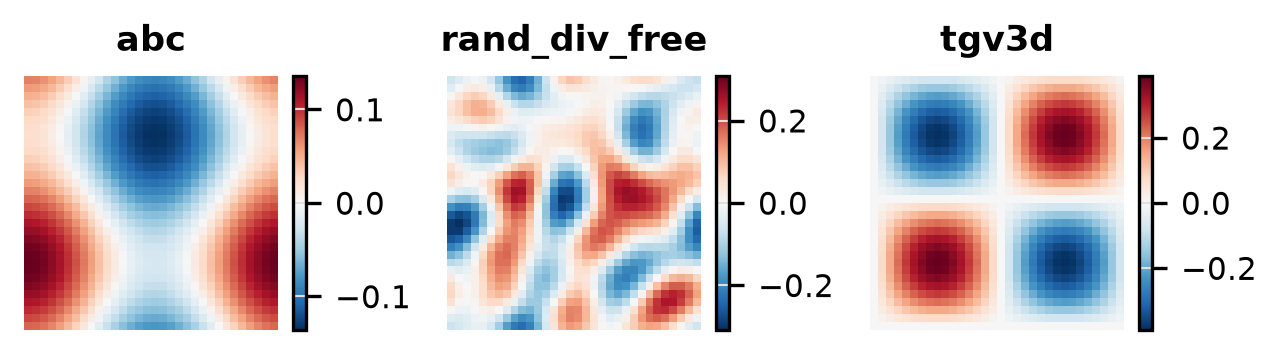
Visualisation of each initial condition (the starting field a run is launched from) available for this problem. IC plots are generated without running any solver.
Abc
{
  "N": 32
}
Rand Div Free
{
  "N": 32
}
Tgv3D
{
  "N": 32
}
Forward
Is the prediction right? Forward-pass benchmarks check each solver’s output against a trusted reference (and an analytic solution where one exists): inter-solver agreement, field-level diagnostics, and long-run stability.
Agreement
3D velocity magnitude fields and kinetic energy spectra per solver, swept over viscosity ν, compared against the analytic TGV reference.
Sweeps nu ∈ {0.001, 0.01, 0.05}
{
  "ic": {
    "name": "tgv3d",
    "seed": 0
  },
  "physics": {
    "N": 16,
    "nu": 0.001,
    "dt": 0.01,
    "steps": 50,
    "lbm_N_base": 16
  },
  "sweep": {
    "key": "nu",
    "values": [
      0.001,
      0.01,
      0.05
    ]
  }
}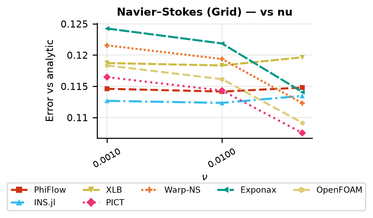
Baseline
Relative error vs grid resolution N at steps=1; validates single-step forward accuracy across 3D solvers.
Sweeps N ∈ {8, 16, 32}
{
  "ic": {
    "name": "tgv3d",
    "seed": 0
  },
  "physics": {
    "N": 8,
    "nu": 0.05,
    "dt": 0.01,
    "steps": 1
  },
  "sweep": {
    "key": "N",
    "values": [
      8,
      16,
      32
    ]
  }
}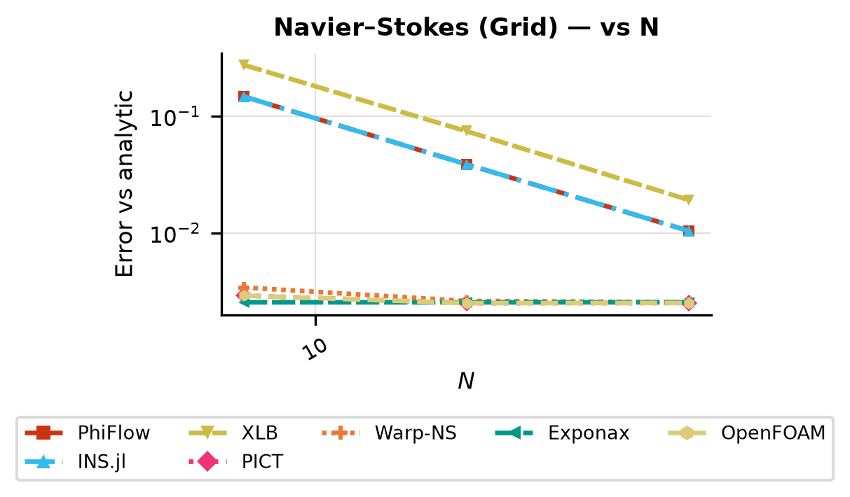
Solver ranking
| Solver | Mean rel. error |
|---|---|
| PICT | 1.13e-01 |
| INS.jl | 1.13e-01 |
| PhiFlow | 1.15e-01 |
| OpenFOAM | 1.15e-01 |
| Warp-NS | 1.18e-01 |
| XLB | 1.19e-01 |
| Exponax | 1.20e-01 |
Ranked by mean relative error against the reference solution (lower is more accurate).
Cost
What does it cost? Wall-clock scaling of the forward and VJP passes with problem size \(N\) and the number of integration steps. Timings come from dedicated runners with no concurrent workloads; see the reliability note at the top of the page before reading absolute numbers.
Spatial Cost
Sweeps N ∈ {16, 32, 48, 64}
{
  "physics": {
    "nu": 0.01,
    "dt": 0.01,
    "lbm_N_base": 16,
    "steps": 50,
    "N": 16
  },
  "cost": {
    "n_trials": 3
  },
  "sweep": {
    "key": "N",
    "values": [
      16,
      32,
      48,
      64
    ]
  }
}
Temporal Cost
Sweeps steps ∈ {10, 50, 100}
{
  "physics": {
    "nu": 0.01,
    "dt": 0.01,
    "lbm_N_base": 16,
    "N": 48,
    "steps": 10
  },
  "cost": {
    "n_trials": 3
  },
  "sweep": {
    "key": "steps",
    "values": [
      10,
      50,
      100
    ]
  }
}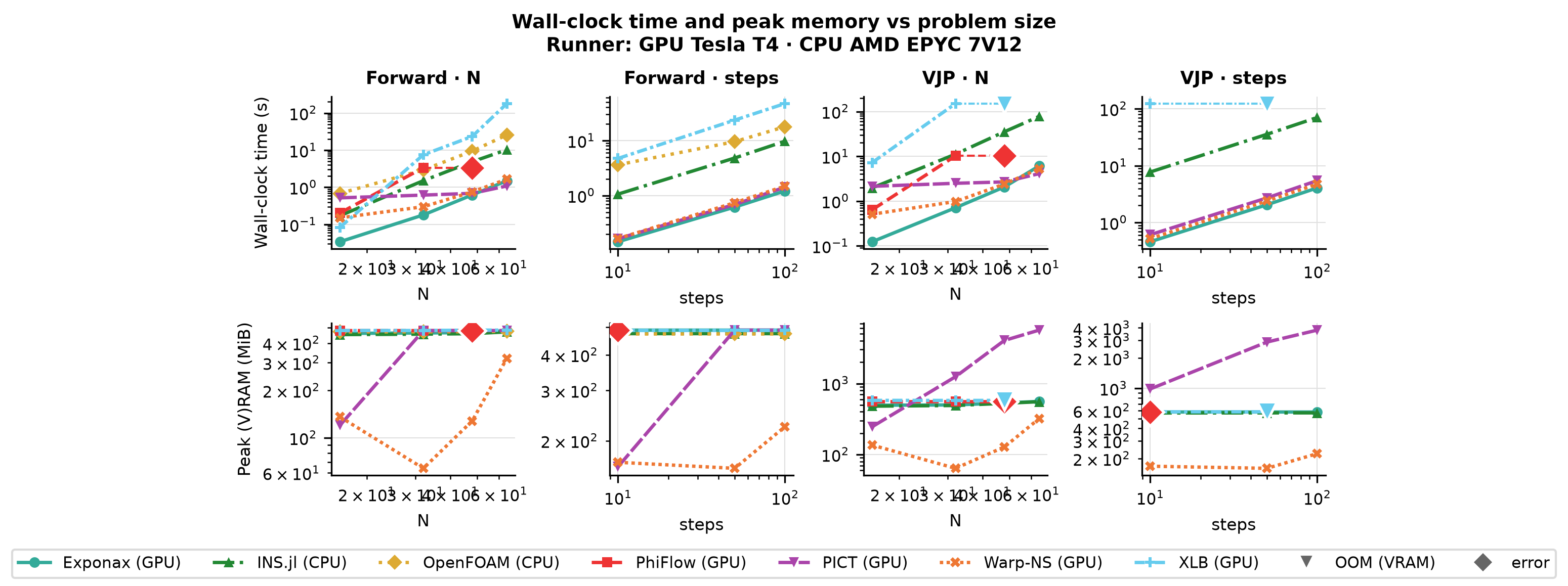
Solver ranking
| Solver | Forward time | VJP time |
|---|---|---|
| PICT | 1.08 s @ N=64 | 4.1 s @ N=64 |
| Exponax | 1.5 s @ N=64 | 6.07 s @ N=64 |
| Warp-NS | 1.66 s @ N=64 | 5.31 s @ N=64 |
| PhiFlow | 3.37 s @ N=32 | 10.3 s @ N=32 |
| INS.jl | 10.3 s @ N=64 | 77.6 s @ N=64 |
| OpenFOAM | 25.8 s @ N=64 | — |
| XLB | 180 s @ N=64 | 151 s @ N=32 |
Forward and VJP (backward) wall-clock time, each shown at the largest problem size N the solver completed for that pass; ranked by forward time (faster is better). Forward-only solvers have no VJP entry. See the reliability note above before comparing across devices.
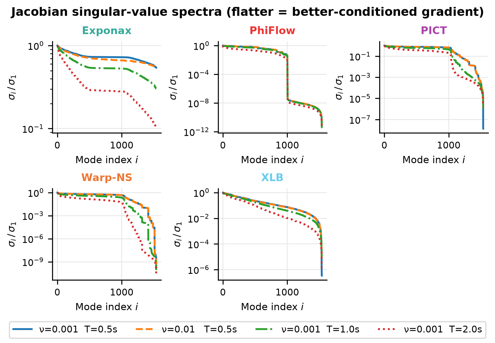
Gradient
Is the gradient right? Gradient benchmarks compare each solver’s AD/adjoint gradient against a finite-difference ground truth. We report magnitude error (relative \(L^2\)) and direction agreement (cosine similarity) across parameter, resolution, and horizon sweeps. The horizon sweep in particular exposes how gradients degrade as the rollout lengthens.
Fd Check
{
  "ic": {
    "name": "tgv3d",
    "seed": 0
  },
  "physics": {
    "N": 16,
    "nu": 0.001,
    "dt": 0.05,
    "steps": 10
  },
  "fd": {
    "eps_values": [
      5.0,
      1.0,
      0.1,
      0.01,
      0.001,
      0.0001
    ],
    "n_dirs": 10
  }
}
Horizon Sweep Limits
Sweeps steps ∈ {40, 80, 160, 320, 640, 1280, 2560, 5120, 10240}
{
  "ic": {
    "name": "tgv3d",
    "seed": 0
  },
  "physics": {
    "N": 20,
    "nu": 0.001,
    "dt": 0.05,
    "steps": 40
  },
  "sweep": {
    "key": "steps",
    "values": [
      40,
      80,
      160,
      320,
      640,
      1280,
      2560,
      5120,
      10240
    ]
  }
}
Jacobian Svd
{
  "ic": {
    "name": "tgv3d",
    "seed": 0
  },
  "physics": {
    "N": 8,
    "nu": 0.001,
    "dt": 0.05,
    "steps": 10
  },
  "jacobian": {
    "n_alphas": 41,
    "alpha_range": 0.3
  }
}
Jacobian Svd Nu01
{
  "ic": {
    "name": "tgv3d",
    "seed": 0
  },
  "physics": {
    "N": 8,
    "nu": 0.01,
    "dt": 0.05,
    "steps": 10
  },
  "jacobian": {
    "n_alphas": 41,
    "alpha_range": 0.3
  }
}
Jacobian Svd Steps20
{
  "ic": {
    "name": "tgv3d",
    "seed": 0
  },
  "physics": {
    "N": 8,
    "nu": 0.001,
    "dt": 0.05,
    "steps": 20
  },
  "jacobian": {
    "n_alphas": 41,
    "alpha_range": 0.3
  }
}
Jacobian Svd Steps40
{
  "ic": {
    "name": "tgv3d",
    "seed": 0
  },
  "physics": {
    "N": 8,
    "nu": 0.001,
    "dt": 0.05,
    "steps": 40
  },
  "jacobian": {
    "n_alphas": 41,
    "alpha_range": 0.3
  }
}
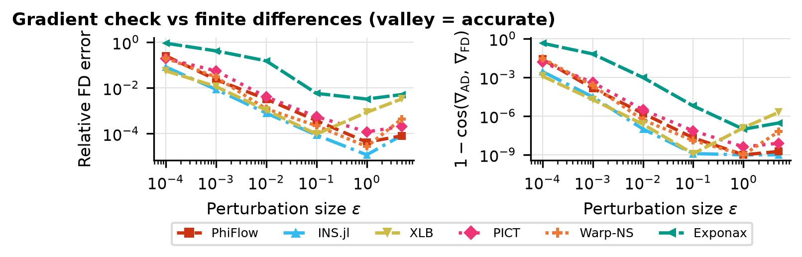
Finite-Difference Check
Finite-difference gradient error U-curves and direction cosine vs perturbation ε for each solver on the 3D Taylor-Green vortex IC.
{
  "ic": {
    "name": "tgv3d",
    "seed": 0
  },
  "physics": {
    "N": 16,
    "nu": 0.001,
    "dt": 0.05,
    "steps": 10
  },
  "fd": {
    "eps_values": [
      5.0,
      1.0,
      0.1,
      0.01,
      0.001,
      0.0001
    ],
    "n_dirs": 10
  }
}
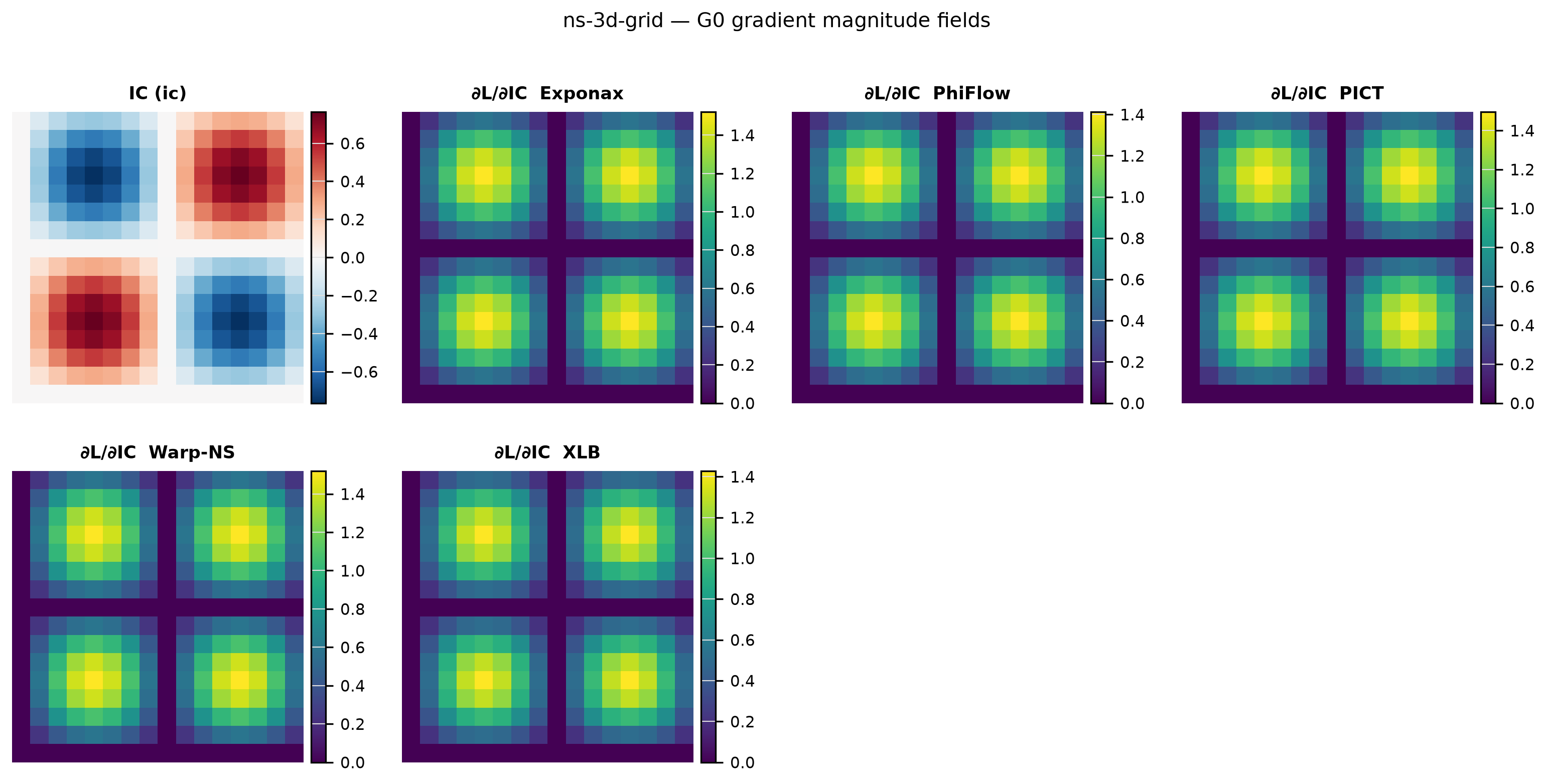
Horizon Sweep Limits
Per-solver rollout-limit table reporting step count at first failure, failure type, and wall time per successful step.
Sweeps steps ∈ {40, 80, 160, 320, 640, 1280, 2560, 5120, 10240}
{
  "ic": {
    "name": "tgv3d",
    "seed": 0
  },
  "physics": {
    "N": 20,
    "nu": 0.001,
    "dt": 0.05,
    "steps": 40
  },
  "sweep": {
    "key": "steps",
    "values": [
      40,
      80,
      160,
      320,
      640,
      1280,
      2560,
      5120,
      10240
    ]
  }
}
Solver ranking
| Solver | Best-ε FD error | 1 − cosine |
|---|---|---|
| INS.jl | 6.01e-06 | 1.58e-11 |
| Warp-NS | 1.30e-05 | 1.58e-10 |
| PhiFlow | 2.62e-05 | 2.81e-10 |
| XLB | 3.71e-05 | 1.23e-09 |
| PICT | 8.39e-05 | 7.90e-09 |
| Exponax | 4.66e-04 | 9.68e-08 |
Ranked by the best-ε finite-difference error of the gradient (lower is more trustworthy); direction cosine near 1 confirms the gradient points the right way.
Optimization
Can you optimize through it? End-to-end optimization benchmarks run a gradient-based optimizer using each solver’s own gradients: recovery of initial conditions or physical parameters, topology optimization, and drag minimization. This is the ultimate test, since a gradient can pass the finite-difference check yet still fail to drive a full optimization loop.
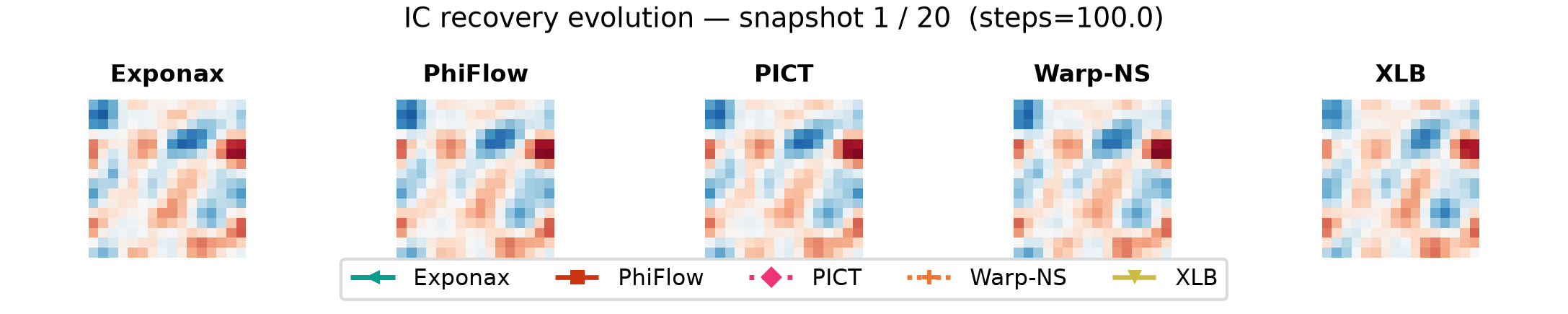
Recovery Constant Ic Bfgs Proj
Final IC recovery error per solver from zero-initialised L-BFGS optimisation with divergence-free projection.
Sweeps steps ∈ {100}
{
  "ic": {
    "name": "rand_div_free",
    "seed": 0
  },
  "physics": {
    "N": 16,
    "nu": 0.01,
    "dt": 0.02,
    "steps": 100
  },
  "optim": {
    "ic_init_type": "zeros",
    "max_iters": 100,
    "patience": 20,
    "failure_threshold": 2.0,
    "snap_interval": 5,
    "ic_seeds": [
      0,
      1,
      2
    ],
    "record_diagnostics": true
  },
  "sweep": {
    "key": "steps",
    "values": [
      100
    ]
  },
  "optimizer": "bfgs_proj",
  "_exp_key": "recovery_constant_ic_bfgs_proj"
}