Navier–Stokes (2D)

Auto-generated 2026-06-25 08:54 UTC  ·  13 plots

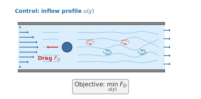
Optimize the inflow of a 2D channel flow to minimize drag on a cylinder, differentiating through an incompressible fluid solver.

Fluid flow in 2D. We simulate an incompressible fluid (think of stirred water) and differentiate through the simulation. The headline question is whether each solver returns a trustworthy gradient as the flow becomes chaotic.

Formally, we solve the 2D incompressible Navier–Stokes equations \(\partial_t \mathbf{u} + (\mathbf{u}\cdot\nabla)\mathbf{u} = -\nabla p + \nu\,\nabla^2\mathbf{u}\), \(\nabla\cdot\mathbf{u}=0\), with the kinematic viscosity \(\nu\) as the primary control parameter. The nonlinear advection term \(\nabla\cdot(\mathbf{u}\otimes\mathbf{u})\) transfers energy across scales; at low \(\nu\) the flow develops turbulent cascades and a positive Lyapunov exponent, so long-horizon gradients grow exponentially sensitive to perturbations. This is the regime where backprop-through-simulation is hardest.

How these results were produced

These are example results, produced automatically on GitHub Actions runners and refreshed on every release. Each solver runs on its intended device: GPU-capable solvers on a Tesla T4 GPU node, CPU-only solvers (OpenFOAM, deal.II, FEniCS, Firedrake) on a CPU node. Accuracy and gradient metrics are hardware-independent and reproducible. Wall-clock numbers reflect commodity cloud hardware and can vary by 10–15% between runs, so read them for relative scaling between solvers rather than as absolute timings. For numbers that reflect your setup, run the benchmarks yourself on your target hardware.

Boundary conditions

Doubly-periodic square domain \([0, 2\pi]^2\) (the flow wraps around at every edge). Incompressibility \(\nabla\cdot\mathbf{u}=0\) is enforced by a pressure projection at each time step. No walls or inflow/outflow boundaries.

Initial Conditions

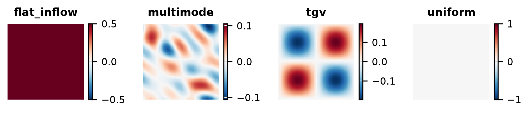
Visualisation of each initial condition (the starting field a run is launched from) available for this problem. IC plots are generated without running any solver.

Settings

Flat Inflow

{
  "N": 64,
  "U": 0.5
}

Multimode

{
  "N": 64
}

Tgv

{
  "N": 64
}

Uniform

{
  "N": 64,
  "U": 1.0
}

Forward

Is the prediction right? Forward-pass benchmarks check each solver’s output against a trusted reference (and an analytic solution where one exists): inter-solver agreement, field-level diagnostics, and long-run stability.

Baseline

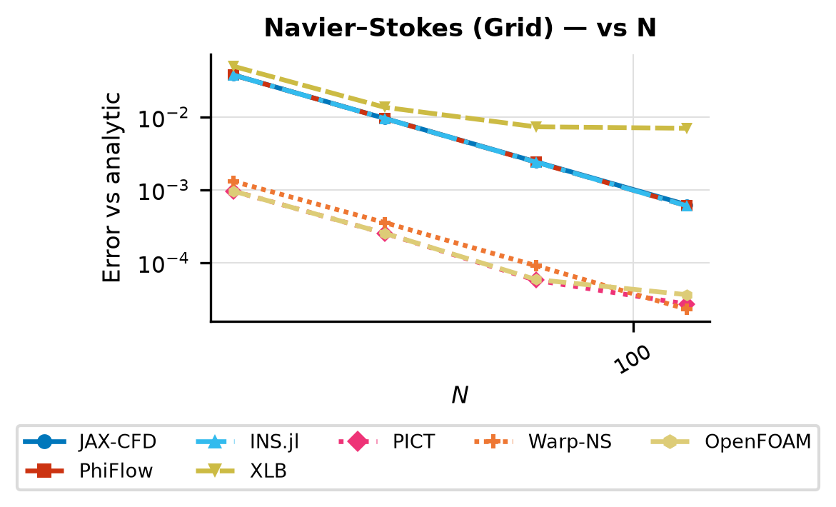
Relative error vs grid resolution \(N\) at steps=1; validates single-step forward accuracy across solvers.

Settings

Sweeps N ∈ {16, 32, 64, 128}

{
  "ic": {
    "name": "tgv",
    "seed": 0
  },
  "physics": {
    "N": 16,
    "nu": 0.05,
    "dt": 0.01,
    "steps": 1,
    "lbm_N_base": 64
  },
  "sweep": {
    "key": "N",
    "values": [
      16,
      32,
      64,
      128
    ]
  }
}

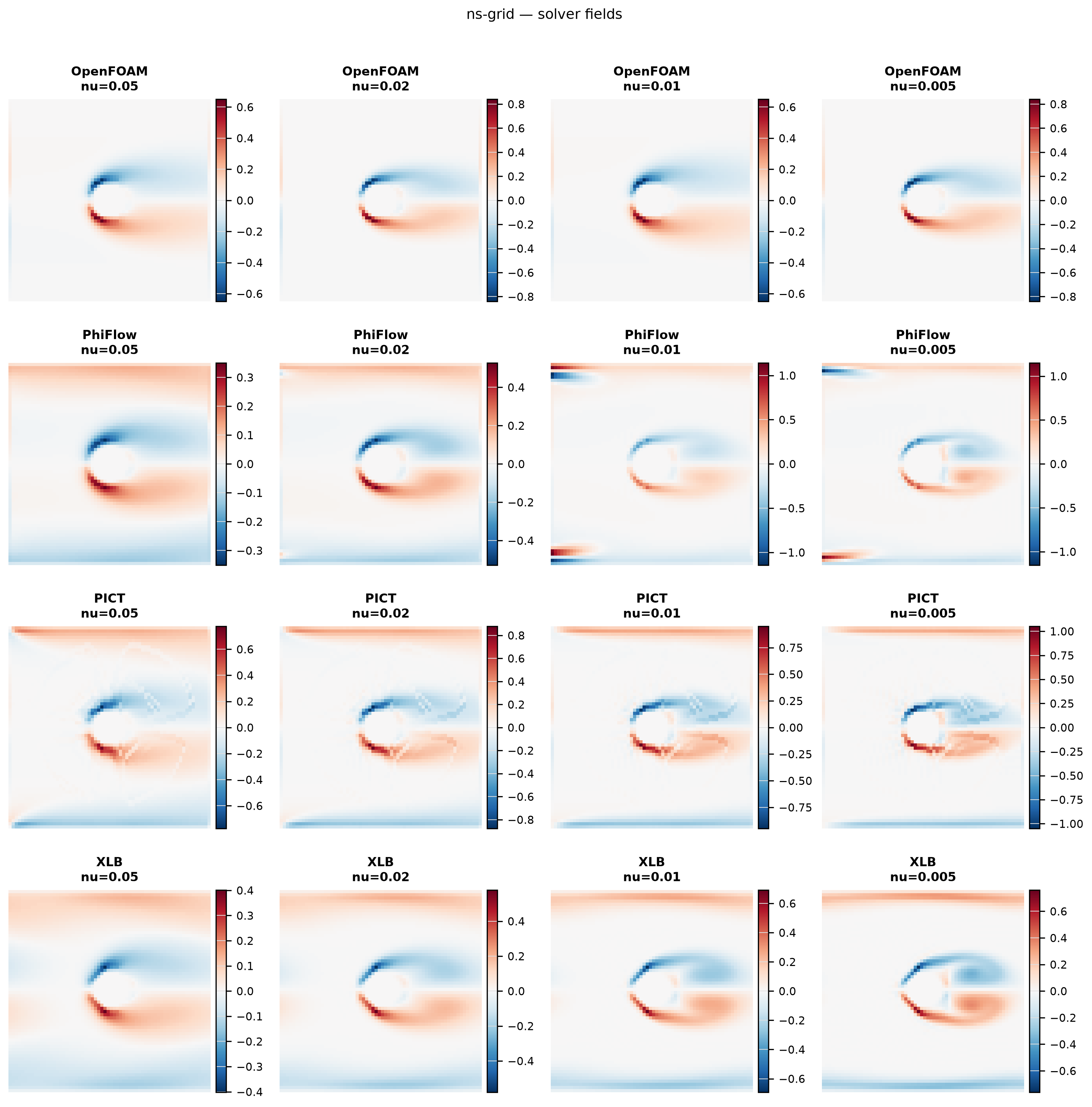
Cylinder

Vorticity snapshots and kinetic-energy evolution vs time for each solver across a sweep of viscosities.

Settings

Sweeps nu ∈ {0.05, 0.02, 0.01, 0.005}

{
  "ic": {
    "name": "uniform",
    "seed": 0
  },
  "physics": {
    "N": 64,
    "dt": 0.01,
    "steps": 500,
    "obstacle": {
      "shape": "cylinder",
      "center": [
        0.5,
        0.5
      ],
      "radius": 0.1
    },
    "nu": 0.05
  },
  "reference_solver": "openfoam",
  "sweep": {
    "key": "nu",
    "values": [
      0.05,
      0.02,
      0.01,
      0.005
    ]
  }
}

Tgv Nu Sweep

Relative error vs viscosity \(\nu\) for each solver at a fixed TGV initial condition.

Settings

Sweeps nu ∈ {0.0001, 0.0005, 0.001, 0.005, 0.01, 0.05}

{
  "ic": {
    "name": "tgv",
    "seed": 42
  },
  "physics": {
    "N": 64,
    "dt": 0.05,
    "steps": 20,
    "nu": 0.0001
  },
  "sweep": {
    "key": "nu",
    "values": [
      0.0001,
      0.0005,
      0.001,
      0.005,
      0.01,
      0.05
    ]
  }
}

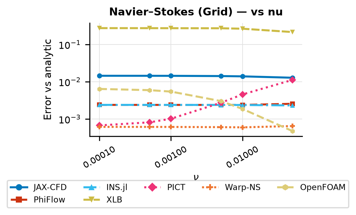
Solver ranking

Solver	Mean rel. error
Warp-NS	6.20e-04
INS.jl	2.39e-03
PhiFlow	2.43e-03
PICT	3.52e-03
OpenFOAM	3.88e-03
jax-cfd	1.41e-02
XLB	2.63e-01

Ranked by mean relative error against the reference solution (lower is more accurate).

Cost

What does it cost? Wall-clock scaling of the forward and VJP passes with problem size \(N\) and the number of integration steps. Timings come from dedicated runners with no concurrent workloads; see the reliability note at the top of the page before reading absolute numbers.

Settings

Spatial Cost

Sweeps N ∈ {64, 128, 192, 256}

{
  "physics": {
    "nu": 0.01,
    "dt": 0.01,
    "steps": 100,
    "N": 64
  },
  "cost": {
    "n_trials": 3
  },
  "sweep": {
    "key": "N",
    "values": [
      64,
      128,
      192,
      256
    ]
  }
}

Temporal Cost

Sweeps steps ∈ {10, 50, 100, 500, 1000}

{
  "physics": {
    "nu": 0.01,
    "dt": 0.01,
    "N": 128,
    "steps": 10
  },
  "cost": {
    "n_trials": 3
  },
  "sweep": {
    "key": "steps",
    "values": [
      10,
      50,
      100,
      500,
      1000
    ]
  }
}

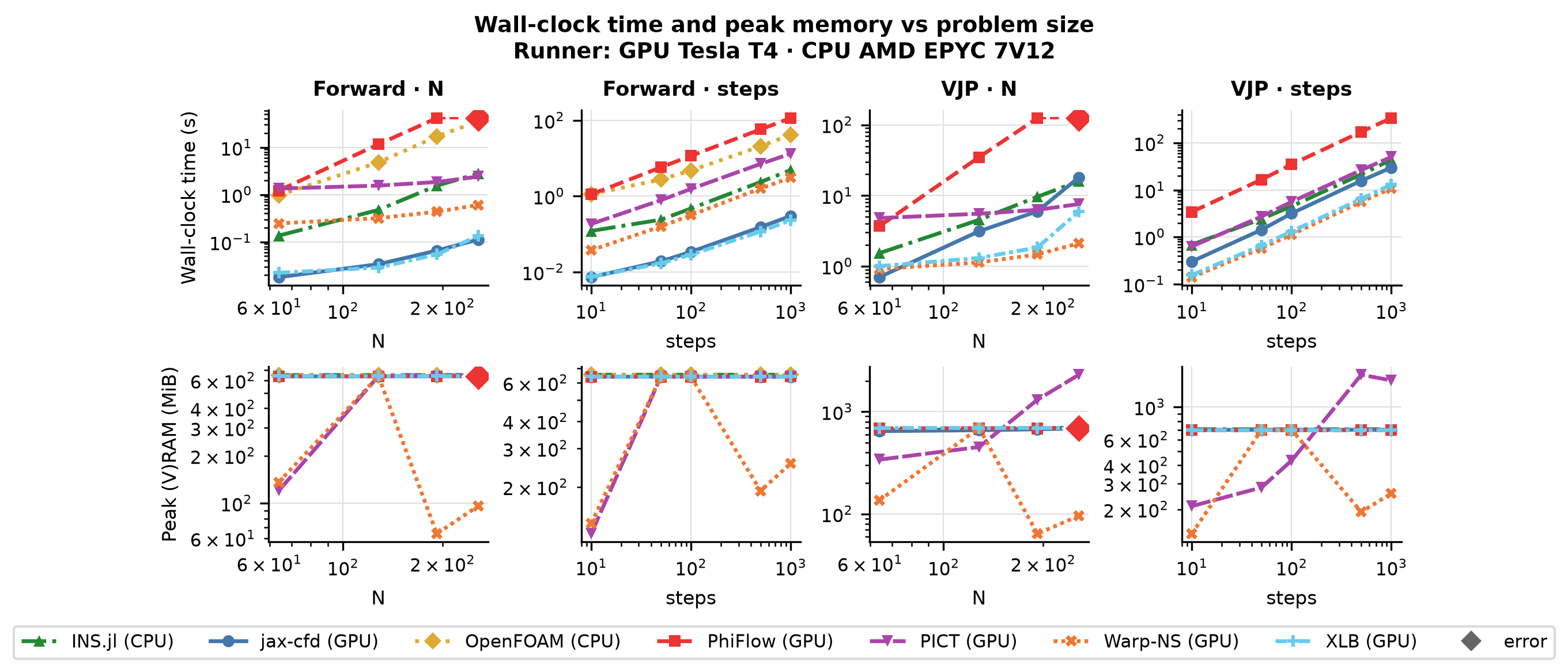
Solver ranking

Solver	Forward time	VJP time
jax-cfd	0.112 s @ N=256	18.1 s @ N=256
XLB	0.134 s @ N=256	5.93 s @ N=256
Warp-NS	0.603 s @ N=256	2.11 s @ N=256
PICT	2.4 s @ N=256	7.57 s @ N=256
INS.jl	2.78 s @ N=256	16 s @ N=256
OpenFOAM	35.4 s @ N=256	—
PhiFlow	41.4 s @ N=192	125 s @ N=192

Forward and VJP (backward) wall-clock time, each shown at the largest problem size N the solver completed for that pass; ranked by forward time (faster is better). Forward-only solvers have no VJP entry. See the reliability note above before comparing across devices.

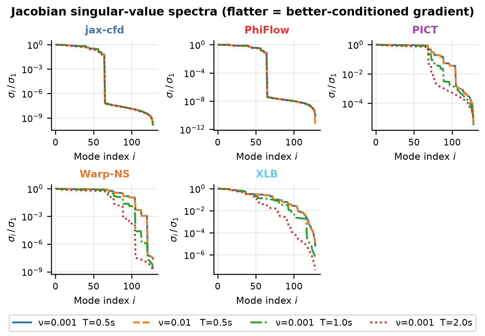
Gradient

Is the gradient right? Gradient benchmarks compare each solver’s AD/adjoint gradient against a finite-difference ground truth. We report magnitude error (relative \(L^2\)) and direction agreement (cosine similarity) across parameter, resolution, and horizon sweeps. The horizon sweep in particular exposes how gradients degrade as the rollout lengthens.

Settings

Fd Check

{
  "ic": {
    "name": "multimode",
    "seed": 42
  },
  "physics": {
    "N": 16,
    "nu": 0.001,
    "dt": 0.05,
    "steps": 20
  },
  "fd": {
    "eps_values": [
      5.0,
      1.0,
      0.1,
      0.01,
      0.001,
      0.0001
    ],
    "n_dirs": 20
  }
}

Horizon Sweep

Sweeps steps ∈ {5, 10, 20, 40, 80, 160, 320}

{
  "ic": {
    "name": "multimode",
    "seed": 42
  },
  "physics": {
    "N": 16,
    "nu": 0.001,
    "dt": 0.05,
    "steps": 5
  },
  "fd": {
    "eps_values": [
      1.0,
      0.1,
      0.01,
      0.001
    ],
    "n_dirs": 8
  },
  "sweep": {
    "key": "steps",
    "values": [
      5,
      10,
      20,
      40,
      80,
      160,
      320
    ]
  }
}

Jacobian Svd

{
  "ic": {
    "name": "multimode",
    "seed": 42
  },
  "physics": {
    "N": 8,
    "nu": 0.001,
    "dt": 0.05,
    "steps": 10
  }
}

Jacobian Svd Nu01

{
  "ic": {
    "name": "multimode",
    "seed": 42
  },
  "physics": {
    "N": 8,
    "nu": 0.01,
    "dt": 0.05,
    "steps": 10
  }
}

Jacobian Svd Steps20

{
  "ic": {
    "name": "multimode",
    "seed": 42
  },
  "physics": {
    "N": 8,
    "nu": 0.001,
    "dt": 0.05,
    "steps": 20
  }
}

Jacobian Svd Steps40

{
  "ic": {
    "name": "multimode",
    "seed": 42
  },
  "physics": {
    "N": 8,
    "nu": 0.001,
    "dt": 0.05,
    "steps": 40
  }
}

Param Sweep

Sweeps nu ∈ {0.05, 0.01, 0.005, 0.001}

{
  "ic": {
    "name": "multimode",
    "seed": 42
  },
  "physics": {
    "N": 16,
    "dt": 0.05,
    "steps": 200,
    "nu": 0.05
  },
  "fd": {
    "eps_values": [
      5.0,
      1.0,
      0.1,
      0.01,
      0.001
    ],
    "n_dirs": 15
  },
  "sweep": {
    "key": "nu",
    "values": [
      0.05,
      0.01,
      0.005,
      0.001
    ]
  }
}

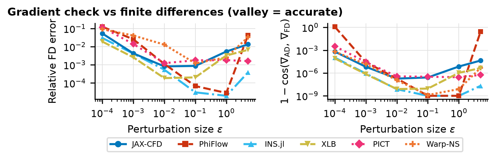
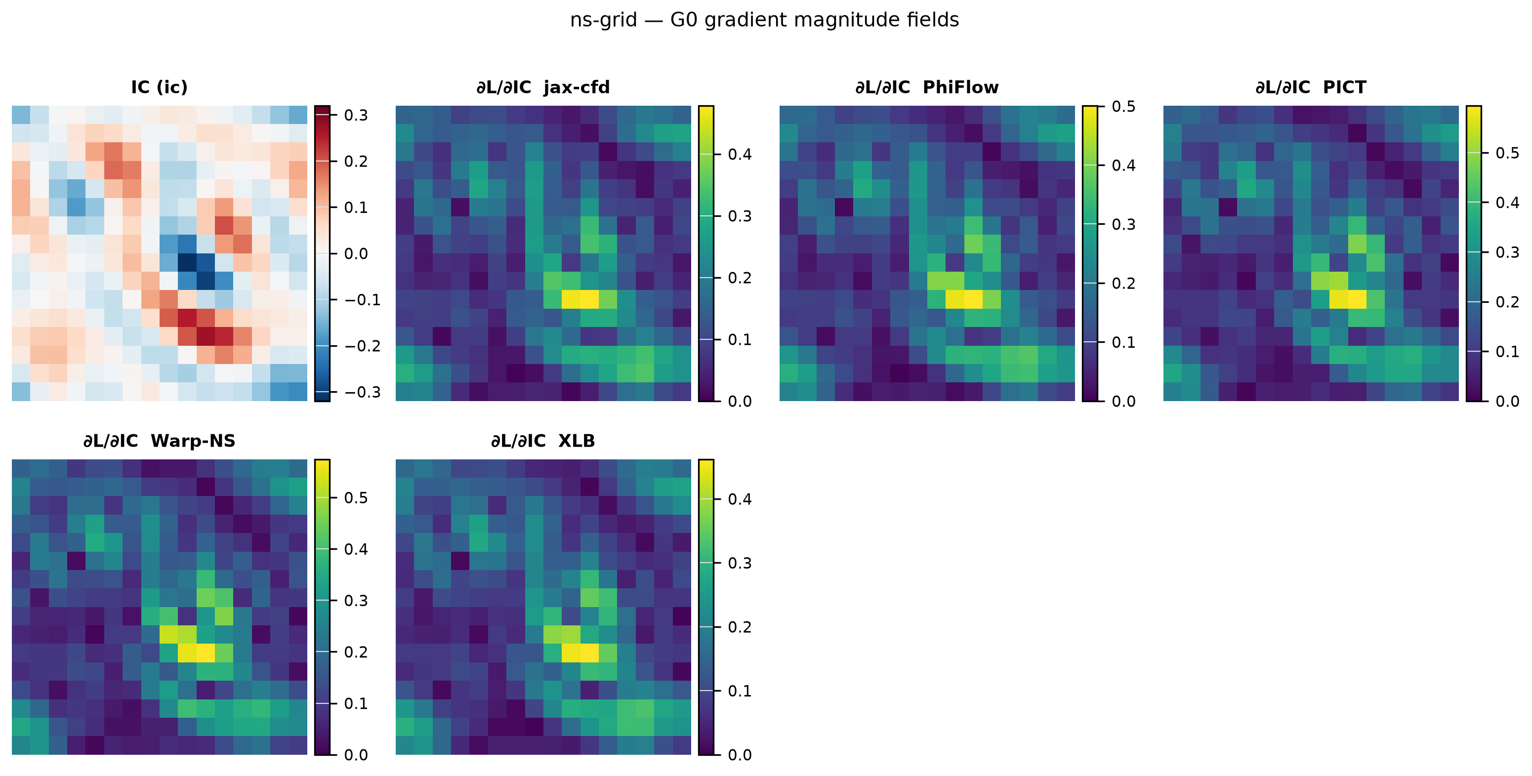
Finite-Difference Check

U-curves of finite-difference gradient error vs perturbation size \(\varepsilon\) together with subspace cosine; validates VJP correctness.

Settings

{
  "ic": {
    "name": "multimode",
    "seed": 42
  },
  "physics": {
    "N": 16,
    "nu": 0.001,
    "dt": 0.05,
    "steps": 20
  },
  "fd": {
    "eps_values": [
      5.0,
      1.0,
      0.1,
      0.01,
      0.001,
      0.0001
    ],
    "n_dirs": 20
  }
}

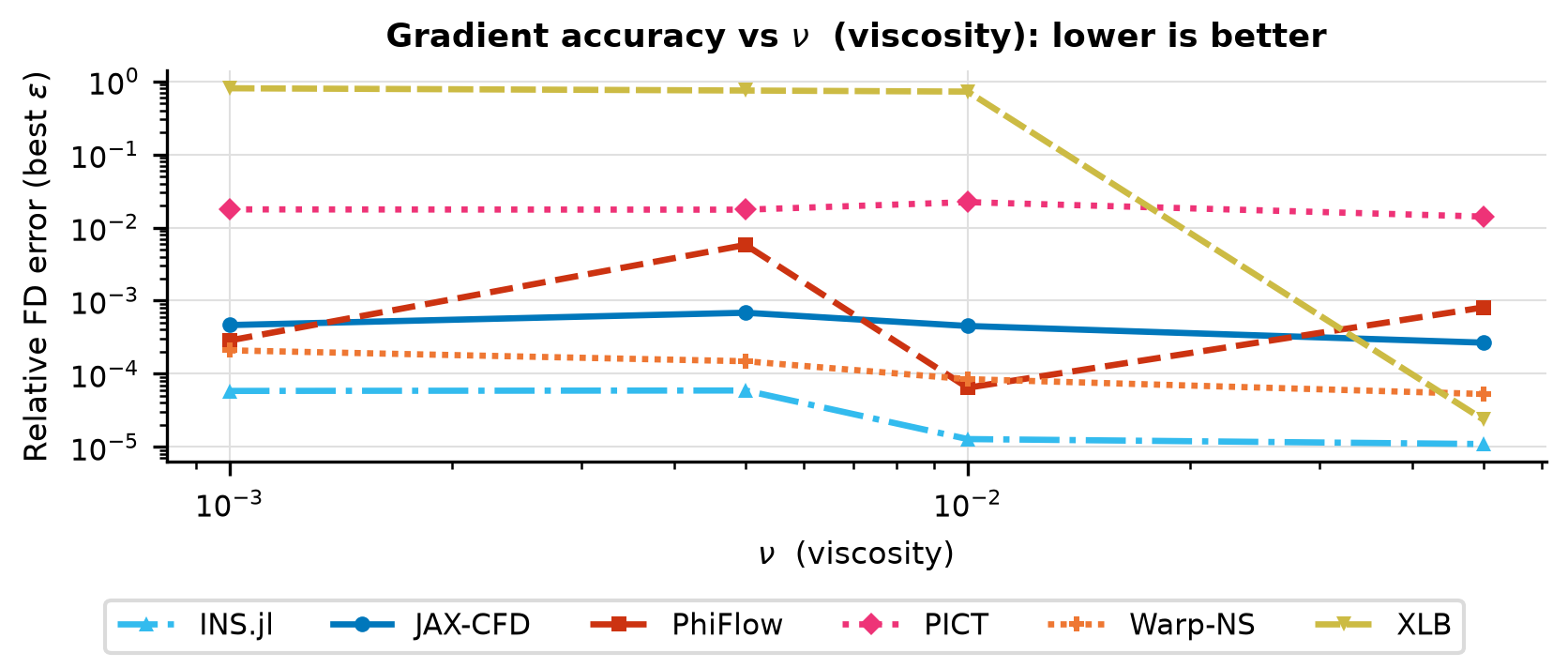
Parameter Sweep

Gradient norm, best-\(\varepsilon\) FD error, direction cosine, and U-curves vs the sweep parameter.

Settings

Sweeps nu ∈ {0.05, 0.01, 0.005, 0.001}

{
  "ic": {
    "name": "multimode",
    "seed": 42
  },
  "physics": {
    "N": 16,
    "dt": 0.05,
    "steps": 200,
    "nu": 0.05
  },
  "fd": {
    "eps_values": [
      5.0,
      1.0,
      0.1,
      0.01,
      0.001
    ],
    "n_dirs": 15
  },
  "sweep": {
    "key": "nu",
    "values": [
      0.05,
      0.01,
      0.005,
      0.001
    ]
  }
}

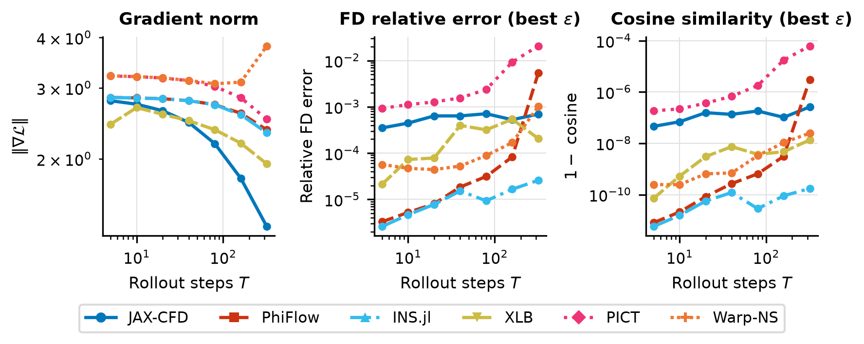
Horizon Sweep

Gradient norm, FD error, and direction cosine vs rollout horizon \(T = \mathrm{steps}\cdot dt\).

Settings

Sweeps steps ∈ {5, 10, 20, 40, 80, 160, 320}

{
  "ic": {
    "name": "multimode",
    "seed": 42
  },
  "physics": {
    "N": 16,
    "nu": 0.001,
    "dt": 0.05,
    "steps": 5
  },
  "fd": {
    "eps_values": [
      1.0,
      0.1,
      0.01,
      0.001
    ],
    "n_dirs": 8
  },
  "sweep": {
    "key": "steps",
    "values": [
      5,
      10,
      20,
      40,
      80,
      160,
      320
    ]
  }
}

Solver ranking

Solver	Best-ε FD error	1 − cosine
PhiFlow	7.44e-06	1.10e-10
INS.jl	7.68e-06	3.38e-11
Warp-NS	4.35e-05	1.26e-09
XLB	8.62e-05	8.89e-09
jax-cfd	5.46e-04	1.84e-07
PICT	8.84e-04	5.62e-07

Ranked by the best-ε finite-difference error of the gradient (lower is more trustworthy); direction cosine near 1 confirms the gradient points the right way.

Optimization

Can you optimize through it? End-to-end optimization benchmarks run a gradient-based optimizer using each solver’s own gradients: recovery of initial conditions or physical parameters, topology optimization, and drag minimization. This is the ultimate test, since a gradient can pass the finite-difference check yet still fail to drive a full optimization loop.

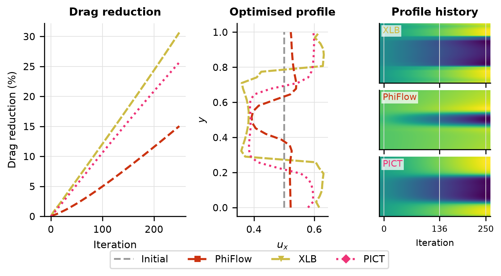
Drag Opt

Drag convergence curves per solver, optimised vs initial inflow profiles, and final drag coefficient comparison.

Settings

{
  "ic": {
    "name": "flat_inflow",
    "seed": 0
  },
  "physics": {
    "N": 32,
    "nu": 0.0025,
    "dt": 0.02,
    "steps": 200,
    "domain_extent": 1.0,
    "U_mean": 0.5,
    "obstacle": {
      "shape": "cylinder",
      "center": [
        0.5,
        0.5
      ],
      "radius": 0.05
    }
  },
  "optim": {
    "lr": 0.0005,
    "max_iters": 250,
    "patience": 50,
    "flow_penalty_weight": 50.0,
    "snap_interval": 20
  }
}

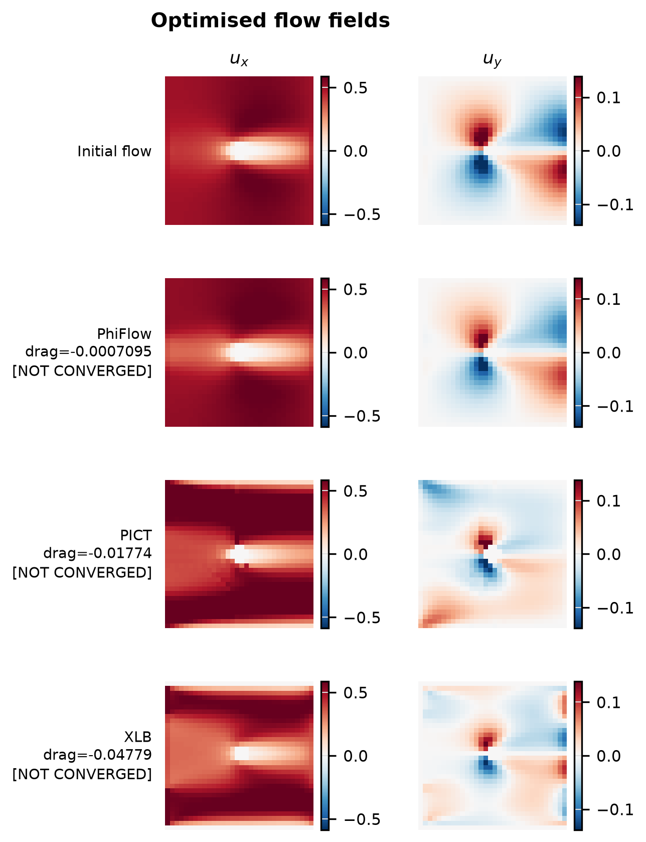
Solver ranking

Solver	Final drag	Converged
XLB	-4.78e-02	no
PICT	-1.77e-02	no
PhiFlow	-7.09e-04	no

Ranked by the final objective reached within the iteration budget (lower is better).