Structural mechanics

Auto-generated 2026-06-25 08:54 UTC  ·  14 plots

Place a fixed budget of material in a clamped beam to make it as stiff as possible, differentiating through a finite-element solve.

Designing a stiff structure. Given a fixed amount of material, where should it go to make a loaded beam as rigid as possible? This is topology optimization, solved by differentiating a finite-element stress analysis with respect to a per-element material density field \(\rho\).

We minimize the compliance (inverse stiffness) of a 3D linear-elastic cantilever beam under the SIMP density-penalization scheme (\(p=3\), \(E_\max = 70{,}000\) MPa). Each element’s stiffness follows the constitutive relation \(E_\text{eff}(\rho) = E_\min + (E_\max - E_\min)\,\rho^3\), and the global stiffness matrix \(K(\rho)\) couples every element to the displacement field. The objective \(C = \mathbf{F}^\top K(\rho)^{-1}\mathbf{F}\) (external work under load \(\mathbf{F}\)) is smooth but non-convex in \(\rho\), so gradient-based optimization drives the design toward sparse, near-binary \(0/1\) material layouts, and the gradient must stay reliable throughout.

How these results were produced

These are example results, produced automatically on GitHub Actions runners and refreshed on every release. Each solver runs on its intended device: GPU-capable solvers on a Tesla T4 GPU node, CPU-only solvers (OpenFOAM, deal.II, FEniCS, Firedrake) on a CPU node. Accuracy and gradient metrics are hardware-independent and reproducible. Wall-clock numbers reflect commodity cloud hardware and can vary by 10–15% between runs, so read them for relative scaling between solvers rather than as absolute timings. For numbers that reflect your setup, run the benchmarks yourself on your target hardware.

Boundary conditions

3D cantilever beam on domain \([0,2]\times[0,1]\times[0,1]\) (HEX8 elements, 2:1:1 aspect). Dirichlet: all nodes at \(x=0\) have zero displacement (clamped wall). Neumann: a prescribed total force is applied to the right face (\(x=2\)), either a uniform downward traction or a concentrated upward corner load depending on the experiment (controlled by the corner_load flag).

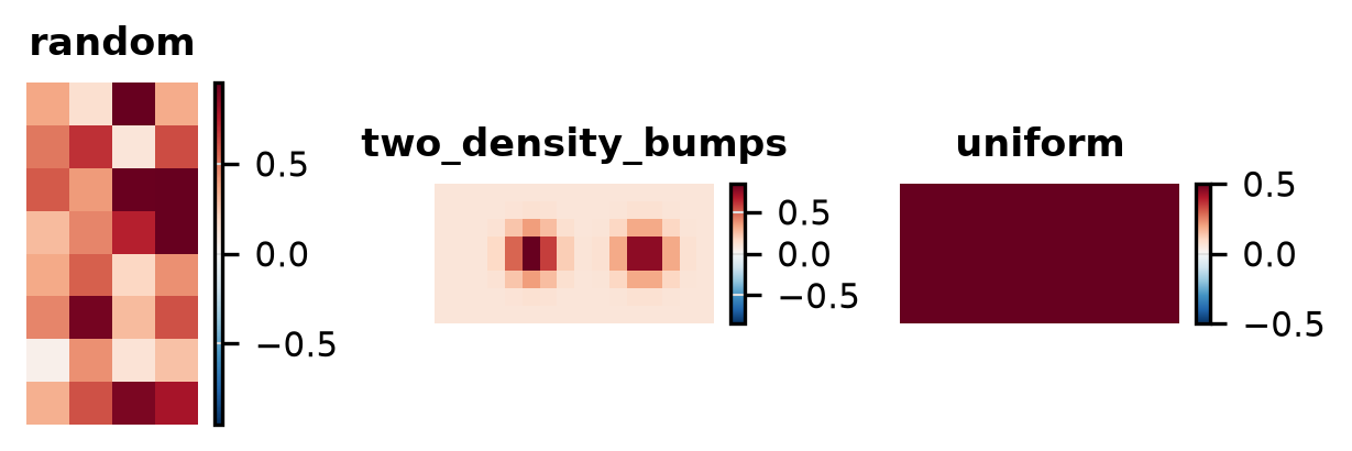
Initial Conditions

Visualisation of each initial condition (the starting field a run is launched from) available for this problem. IC plots are generated without running any solver.

Settings

Two Density Bumps

{
  "nx": 16,
  "ny": 2,
  "nz": 8
}

Uniform

{
  "rho_0": 0.5,
  "nx": 16
}

Forward

Is the prediction right? Forward-pass benchmarks check each solver’s output against a trusted reference (and an analytic solution where one exists): inter-solver agreement, field-level diagnostics, and long-run stability.

Agreement

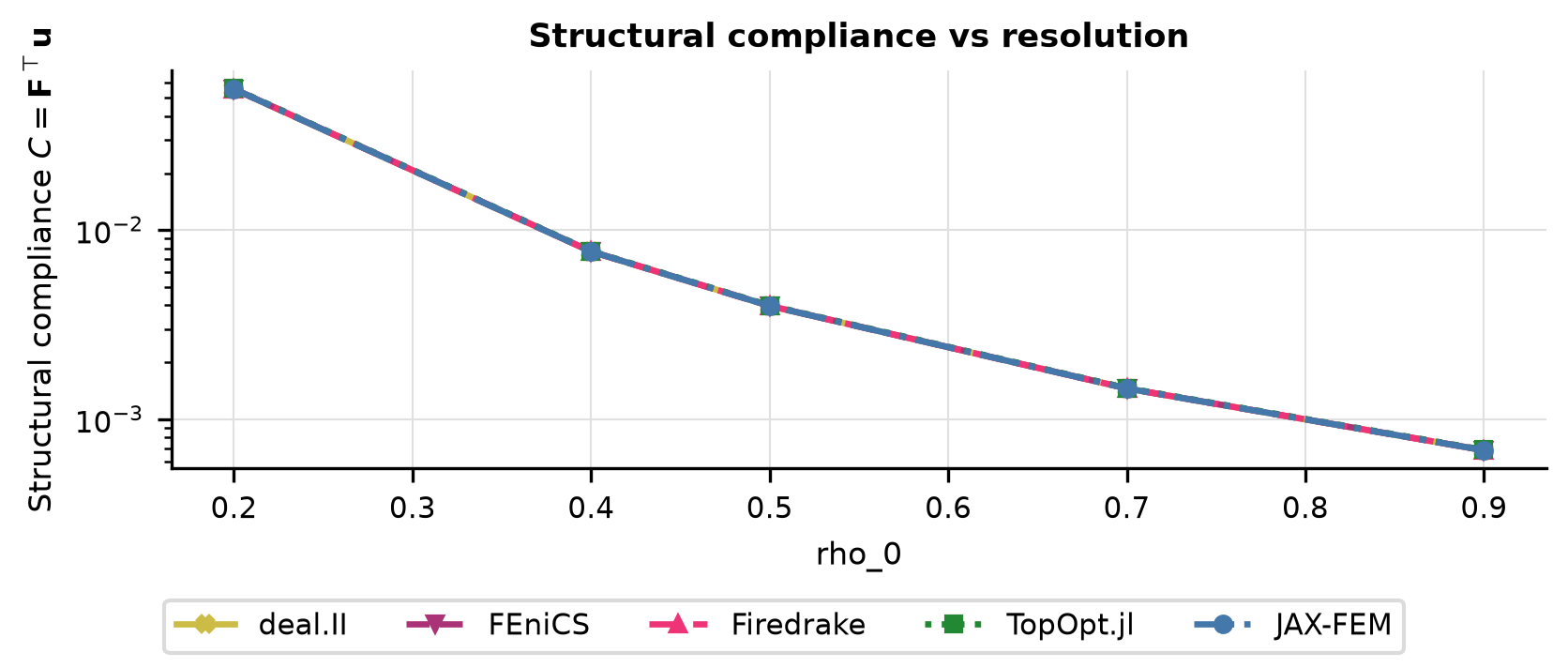
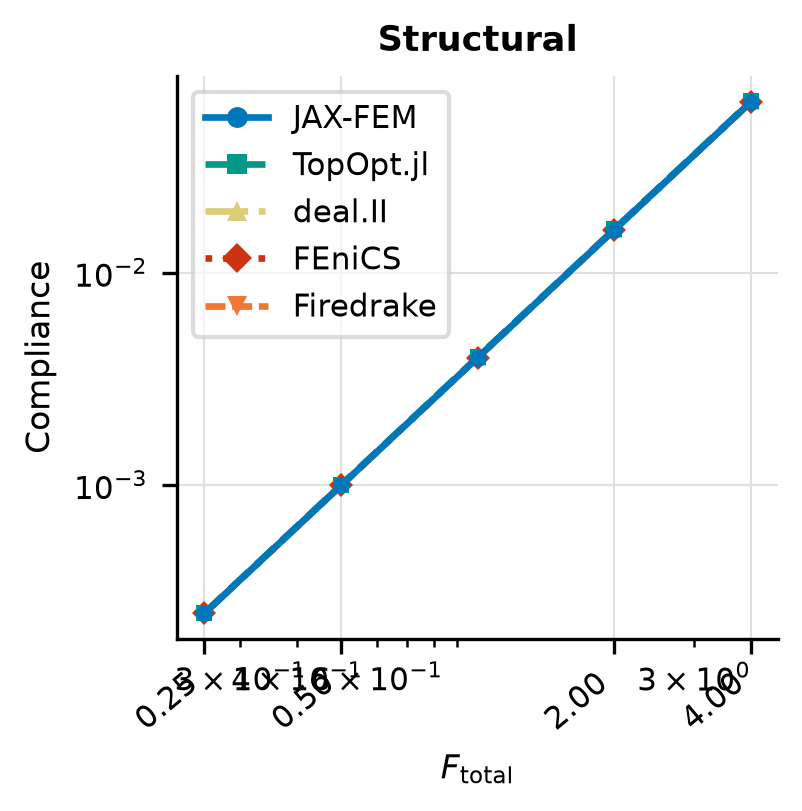
Structural compliance \(C = \mathbf{F}^\top \mathbf{u}\) vs density \(\rho_0\) at fixed mesh, sweeping uniform density to span the SIMP stiffness regime.

Settings

Sweeps rho_0 ∈ {0.2, 0.4, 0.5, 0.7, 0.9}

{
  "ic": {
    "name": "uniform",
    "seed": 0
  },
  "physics": {
    "nx": 8,
    "ny": 2,
    "nz": 4,
    "Lx": 2.0,
    "Ly": 1.0,
    "Lz": 1.0,
    "F_total": 1.0,
    "corner_load": false,
    "rho_0": 0.2
  },
  "sweep": {
    "key": "rho_0",
    "values": [
      0.2,
      0.4,
      0.5,
      0.7,
      0.9
    ]
  }
}

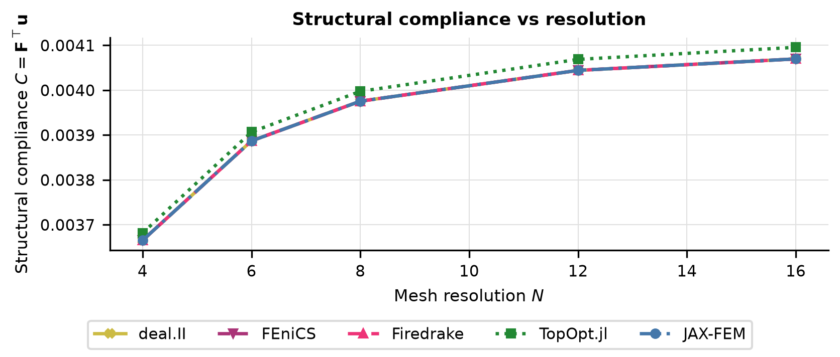
Baseline

Structural compliance \(C = \mathbf{F}^\top \mathbf{u}\) vs mesh resolution \(N\) for each solver, uniform density \(\rho_0=0.5\), full-face downward load.

Settings

Sweeps N ∈ {4, 6, 8, 12, 16}

{
  "ic": {
    "name": "uniform",
    "seed": 0
  },
  "physics": {
    "N": 4,
    "ny": 2,
    "nz": 4,
    "Lx": 2.0,
    "Ly": 1.0,
    "Lz": 1.0,
    "F_total": 1.0,
    "corner_load": false
  },
  "sweep": {
    "key": "N",
    "values": [
      4,
      6,
      8,
      12,
      16
    ]
  }
}

Physical Laws

Diagnostic functionals (compliance, total displacement) vs total load \(F_\mathrm{total}\), validating linearity of the SIMP response.

Settings

Sweeps F_total ∈ {0.25, 0.5, 1.0, 2.0, 4.0}

{
  "ic": {
    "name": "uniform",
    "seed": 0
  },
  "physics": {
    "nx": 8,
    "ny": 2,
    "nz": 4,
    "Lx": 2.0,
    "Ly": 1.0,
    "Lz": 1.0,
    "corner_load": false,
    "rho_0": 0.5,
    "F_total": 0.25
  },
  "sweep": {
    "key": "F_total",
    "values": [
      0.25,
      0.5,
      1.0,
      2.0,
      4.0
    ]
  },
  "diagnostics": {
    "compliance": "<callable _get_compliance>"
  }
}

Solver ranking

Solver	Mean rel. error
deal.II	0
FEniCS	0
Firedrake	0
JAX-FEM	0
TopOpt.jl	5.53e-03

Ranked by mean relative error against the reference solution (lower is more accurate).

Cost

What does it cost? Wall-clock scaling of the forward and VJP passes with problem size \(N\) and the number of integration steps. Timings come from dedicated runners with no concurrent workloads; see the reliability note at the top of the page before reading absolute numbers.

Settings

Spatial Cost

Sweeps nx ∈ {4, 6, 8, 12, 16}

{
  "physics": {
    "Lx": 2.0,
    "Ly": 1.0,
    "Lz": 1.0,
    "F_total": 1.0,
    "rho_0": 0.5,
    "corner_load": false,
    "steps": 1,
    "nx": 4
  },
  "cost": {
    "n_trials": 3
  },
  "sweep": {
    "key": "nx",
    "values": [
      4,
      6,
      8,
      12,
      16
    ]
  }
}

Temporal Cost

Sweeps steps ∈ {1}

{
  "physics": {
    "Lx": 2.0,
    "Ly": 1.0,
    "Lz": 1.0,
    "F_total": 1.0,
    "rho_0": 0.5,
    "corner_load": false,
    "nx": 8,
    "steps": 1
  },
  "cost": {
    "n_trials": 3
  },
  "sweep": {
    "key": "steps",
    "values": [
      1
    ]
  }
}

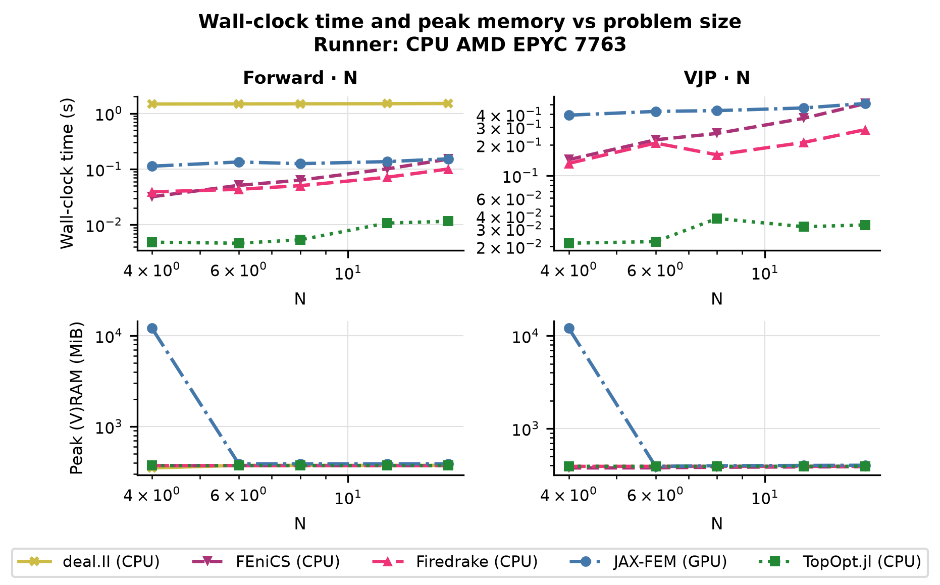
Solver ranking

Solver	Forward time	VJP time
TopOpt.jl	0.0116 s @ N=16	0.0327 s @ N=16
Firedrake	0.101 s @ N=16	0.283 s @ N=16
FEniCS	0.151 s @ N=16	0.51 s @ N=16
JAX-FEM	0.153 s @ N=16	0.511 s @ N=16
deal.II	1.51 s @ N=16	—

Forward and VJP (backward) wall-clock time, each shown at the largest problem size N the solver completed for that pass; ranked by forward time (faster is better). Forward-only solvers have no VJP entry. See the reliability note above before comparing across devices.

Gradient

Is the gradient right? Gradient benchmarks compare each solver’s AD/adjoint gradient against a finite-difference ground truth. We report magnitude error (relative \(L^2\)) and direction agreement (cosine similarity) across parameter, resolution, and horizon sweeps. The horizon sweep in particular exposes how gradients degrade as the rollout lengthens.

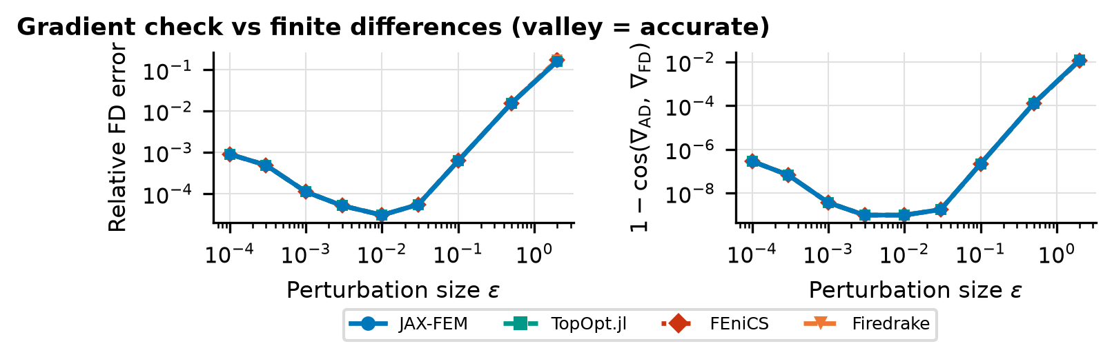
Finite-Difference Check

U-curves of finite-difference gradient error vs perturbation size \(\varepsilon\) with subspace cosine, validating VJP correctness on a random density.

Settings

{
  "ic": {
    "name": "random",
    "seed": 0
  },
  "physics": {
    "nx": 8,
    "ny": 2,
    "nz": 4,
    "Lx": 2.0,
    "Ly": 1.0,
    "Lz": 1.0,
    "F_total": 1.0,
    "corner_load": true
  },
  "fd": {
    "eps_values": [
      2.0,
      0.5,
      0.1,
      0.03,
      0.01,
      0.003,
      0.001,
      0.0003,
      0.0001
    ],
    "n_dirs": 6
  }
}

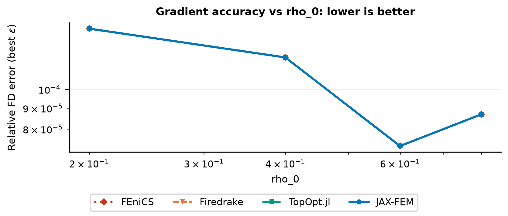
Parameter Sweep

Gradient norm, best-\(\varepsilon\) FD error, direction cosine, and U-curves vs uniform density \(\rho_0\).

Settings

Sweeps rho_0 ∈ {0.2, 0.4, 0.6, 0.8}

{
  "ic": {
    "name": "uniform",
    "seed": 0
  },
  "physics": {
    "nx": 8,
    "ny": 2,
    "nz": 4,
    "Lx": 2.0,
    "Ly": 1.0,
    "Lz": 1.0,
    "F_total": 1.0,
    "corner_load": true,
    "rho_0": 0.2
  },
  "fd": {
    "eps_values": [
      0.5,
      0.1,
      0.03,
      0.01,
      0.003,
      0.001,
      0.0003
    ],
    "n_dirs": 6
  },
  "sweep": {
    "key": "rho_0",
    "values": [
      0.2,
      0.4,
      0.6,
      0.8
    ]
  }
}

Solver ranking

Solver	Best-ε FD error	1 − cosine
FEniCS	2.11e-05	1.97e-10
Firedrake	2.11e-05	1.97e-10
TopOpt.jl	2.11e-05	1.97e-10
JAX-FEM	2.11e-05	1.97e-10

Ranked by the best-ε finite-difference error of the gradient (lower is more trustworthy); direction cosine near 1 confirms the gradient points the right way.

Optimization

Can you optimize through it? End-to-end optimization benchmarks run a gradient-based optimizer using each solver’s own gradients: recovery of initial conditions or physical parameters, topology optimization, and drag minimization. This is the ultimate test, since a gradient can pass the finite-difference check yet still fail to drive a full optimization loop.

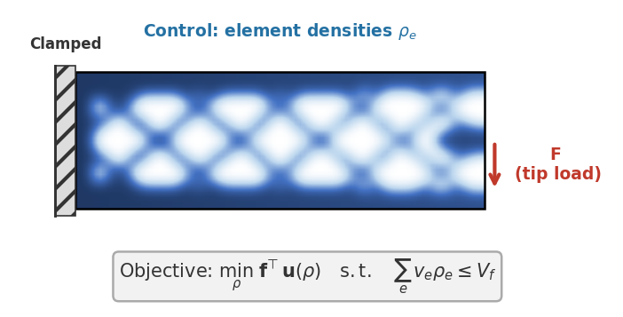
Topology Optimisation

SIMP topology optimisation on a \(16\times8\times8\) cantilever beam with Adam (lr=0.05): compliance \(C = \mathbf{F}^\top \mathbf{u}\) and density field evolution under a 50% volume-fraction constraint.

Settings

{
  "ic": {
    "name": "uniform",
    "seed": 0
  },
  "physics": {
    "nx": 16,
    "ny": 2,
    "nz": 8,
    "Lx": 2.0,
    "Ly": 1.0,
    "Lz": 1.0,
    "F_total": 1.0,
    "corner_load": true,
    "v_frac": 0.5,
    "compliance_key": "compliance",
    "penalty_weight": 50.0,
    "x_min": 0.001,
    "snap_interval": 5
  },
  "optim": {
    "lr": 0.05,
    "max_iters": 2500,
    "patience": 100
  }
}

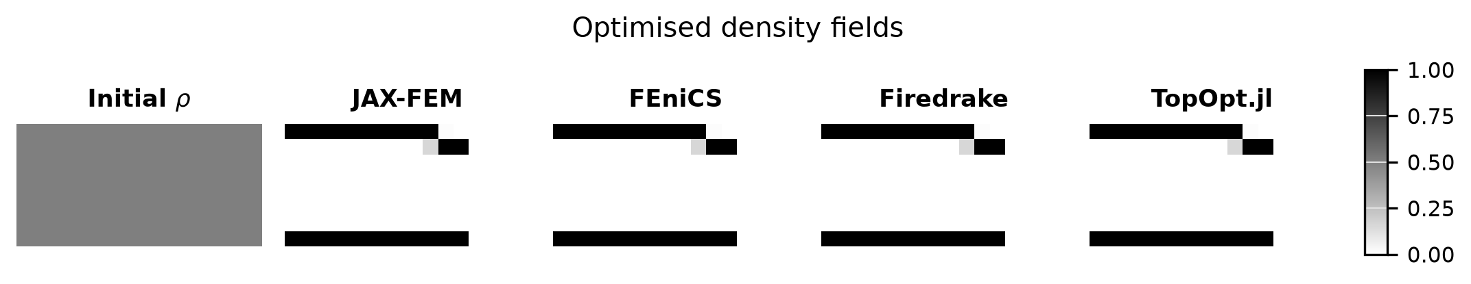
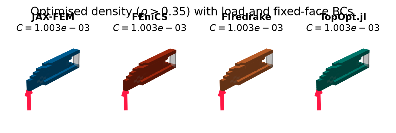
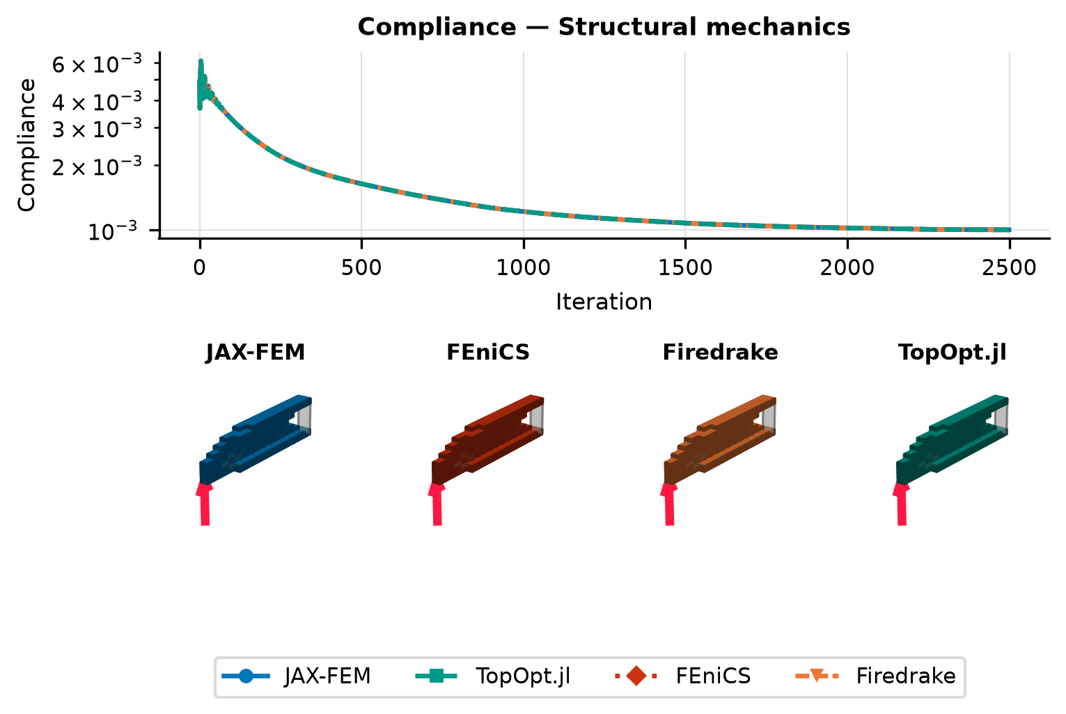
Solver ranking

Solver	Final compliance	Converged
JAX-FEM	1.00e-03	no
FEniCS	1.00e-03	no
Firedrake	1.00e-03	no
TopOpt.jl	1.00e-03	no

Ranked by the final objective reached within the iteration budget (lower is better).