Heat transfer

Auto-generated 2026-06-25 08:54 UTC  ·  12 plots

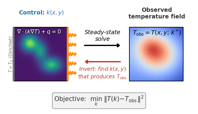
Invert for the conductivity field of a slab from its temperature, differentiating through a steady heat-conduction solve.

Routing heat through a material. Where should the conductive material go to carry heat away most effectively? And, separately, can we recover an unknown heat source from temperature measurements? Both are inverse problems solved by differentiating through a steady heat-conduction solve.

We minimize the thermal compliance of a quasi-2D heated slab under the SIMP density-penalization scheme (\(p=3\)). The effective conductivity \(k_\text{eff}(\rho) = k_\min + (k_\max - k_\min)\,\rho^3\) controls how heat is routed, and the compliance \(C = \oint_\Gamma q_n\,T\,d\Gamma\) measures the work done by the heat flux on the temperature field. A hot-spot boundary condition (a central \(1/3\) stripe) breaks \(y\)-symmetry and drives the topology optimization toward non-trivial branching structures. The same domain also hosts source-identification experiments, which recover an unknown volumetric heat source \(f(\mathbf{x})\) from temperature observations by minimizing \(\lVert T - T_\text{target} \rVert^2\).

How these results were produced

These are example results, produced automatically on GitHub Actions runners and refreshed on every release. Each solver runs on its intended device: GPU-capable solvers on a Tesla T4 GPU node, CPU-only solvers (OpenFOAM, deal.II, FEniCS, Firedrake) on a CPU node. Accuracy and gradient metrics are hardware-independent and reproducible. Wall-clock numbers reflect commodity cloud hardware and can vary by 10–15% between runs, so read them for relative scaling between solvers rather than as absolute timings. For numbers that reflect your setup, run the benchmarks yourself on your target hardware.

Boundary conditions

Quasi-2D heated slab on domain \([0,2]\times[0,1]\) (a single HEX8 layer, \(n_z=1\)). Dirichlet: all nodes at \(x=0\) held at \(T=0\) (fixed temperature). Neumann (uniform): uniform heat flux \(Q_\text{total}\) over the right face (\(x=2\)). Neumann (hot-spot): flux concentrated on the central \(1/3\) stripe in \(y\) (\(L_y/3 \le y \le 2L_y/3\)) at the right face, driving non-trivial topology.

Initial Conditions

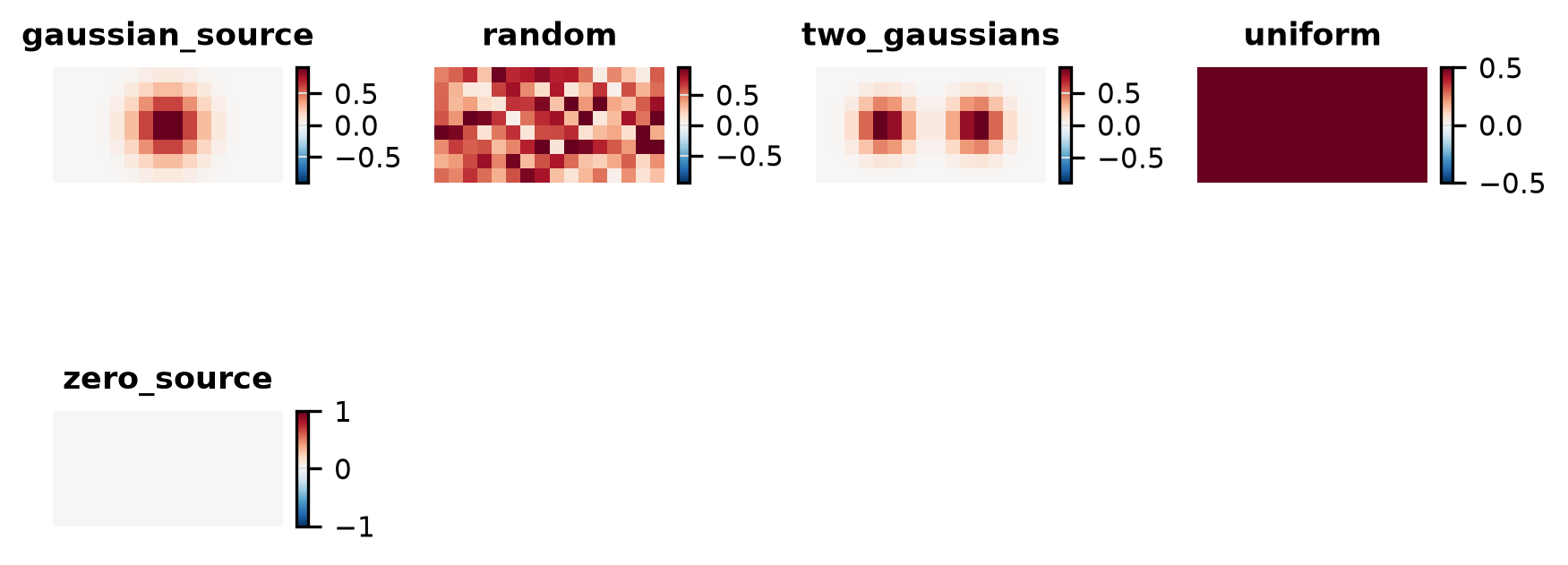
Visualisation of each initial condition (the starting field a run is launched from) available for this problem. IC plots are generated without running any solver.

Settings

Gaussian Source

{
  "nx": 16,
  "ny": 8,
  "nz": 1,
  "amplitude": 1.0,
  "cx": 0.5,
  "cy": 0.5,
  "sigma": 0.2
}

Random

{
  "rho_0": 0.5,
  "noise": 0.3,
  "nx": 16,
  "ny": 8,
  "nz": 1,
  "seed": 0
}

Two Gaussians

{
  "nx": 16,
  "ny": 8,
  "nz": 1
}

Uniform

{
  "rho_0": 0.5,
  "nx": 16,
  "ny": 8,
  "nz": 1
}

Zero Source

{
  "nx": 16,
  "ny": 8,
  "nz": 1
}

Forward

Is the prediction right? Forward-pass benchmarks check each solver’s output against a trusted reference (and an analytic solution where one exists): inter-solver agreement, field-level diagnostics, and long-run stability.

Agreement

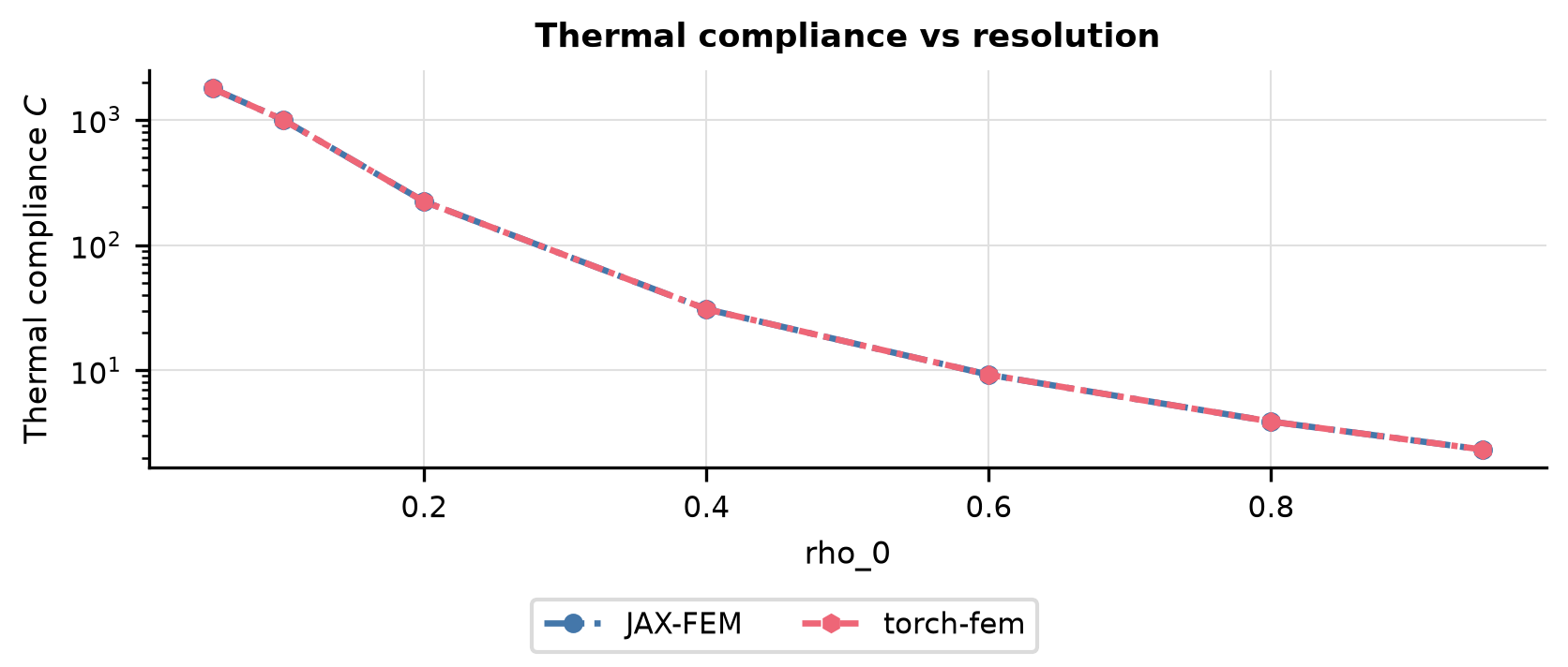
Thermal compliance \(C\) vs uniform element density \(\rho_0\) at fixed \(N\); compares solvers on a log scale.

Settings

Sweeps rho_0 ∈ {0.05, 0.1, 0.2, 0.4, 0.6, 0.8, 0.95}

{
  "ic": {
    "name": "uniform",
    "seed": 0
  },
  "physics": {
    "nx": 16,
    "ny": 8,
    "nz": 1,
    "Lx": 2.0,
    "Ly": 1.0,
    "Lz": 1.0,
    "Q_total": 1.0,
    "rho_0": 0.05
  },
  "sweep": {
    "key": "rho_0",
    "values": [
      0.05,
      0.1,
      0.2,
      0.4,
      0.6,
      0.8,
      0.95
    ]
  }
}

Baseline

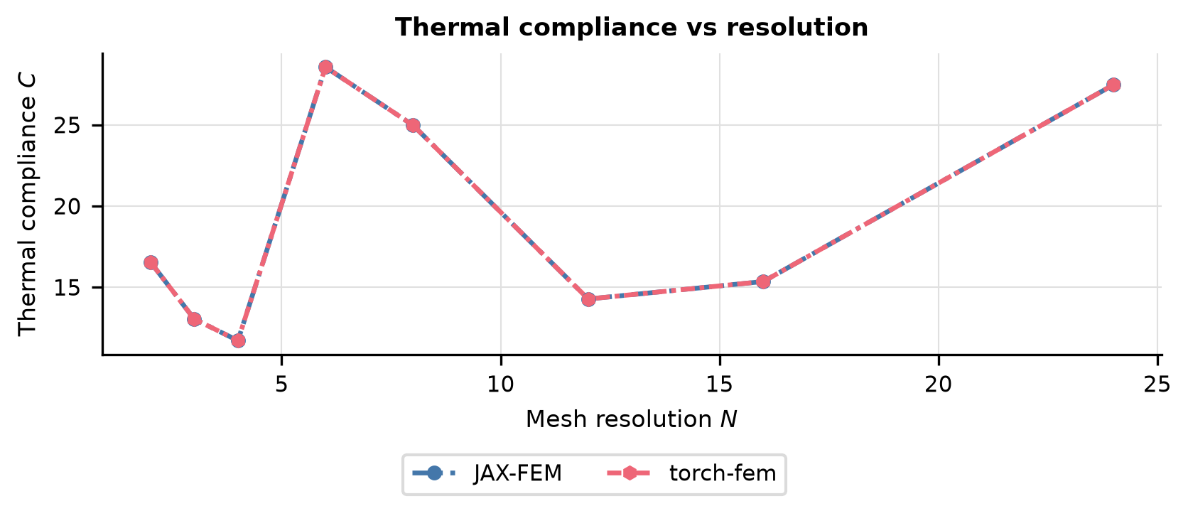
Thermal compliance \(C\) vs mesh resolution \(N\) with random density; compares FV and FEM solvers across refinements.

Settings

Sweeps N ∈ {2, 3, 4, 6, 8, 12, 16, 24}

{
  "ic": {
    "name": "random",
    "seed": 0
  },
  "physics": {
    "N": 2,
    "nz": 1,
    "Lx": 2.0,
    "Ly": 1.0,
    "Lz": 1.0,
    "Q_total": 1.0
  },
  "sweep": {
    "key": "N",
    "values": [
      2,
      3,
      4,
      6,
      8,
      12,
      16,
      24
    ]
  }
}

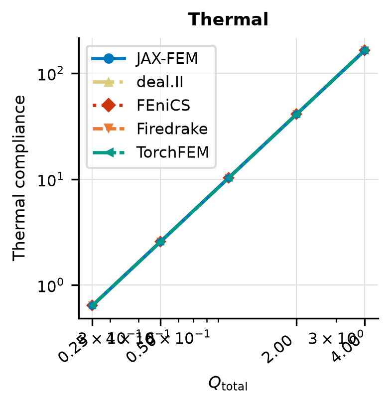
Physical Laws

Thermal compliance \(C\) vs total heat flux \(Q_\mathrm{total}\) at fixed \(N\) and \(\rho_0\) with a hot-spot BC; shown on log-log axes.

Settings

Sweeps Q_total ∈ {0.25, 0.5, 1.0, 2.0, 4.0}

{
  "ic": {
    "name": "uniform",
    "seed": 0
  },
  "physics": {
    "N": 16,
    "nz": 1,
    "Lx": 2.0,
    "Ly": 1.0,
    "Lz": 1.0,
    "rho_0": 0.5,
    "hot_spot": true,
    "Q_total": 0.25
  },
  "sweep": {
    "key": "Q_total",
    "values": [
      0.25,
      0.5,
      1.0,
      2.0,
      4.0
    ]
  },
  "diagnostics": {
    "thermal_compliance": "<callable _get_thermal_compliance>"
  }
}

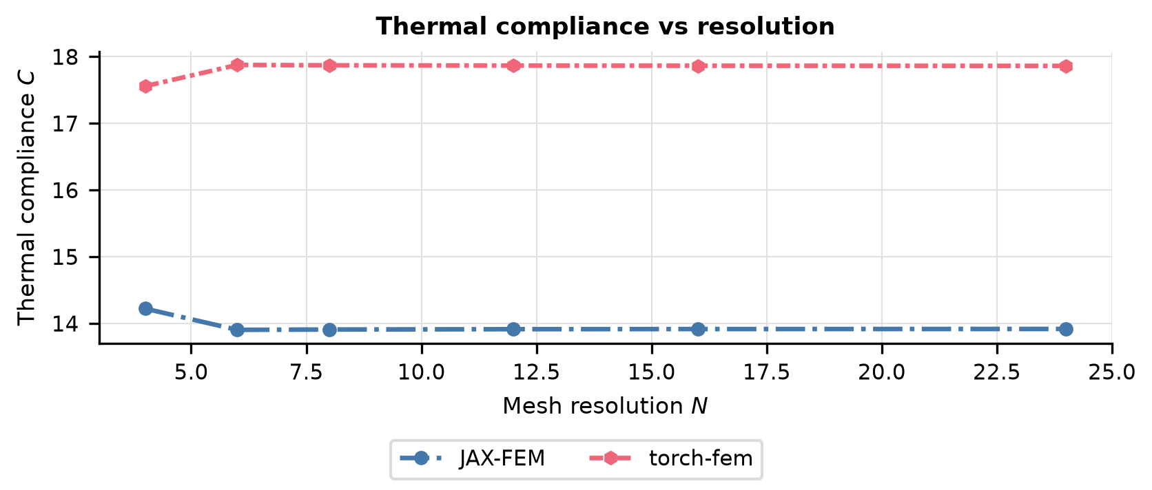
Source Baseline

Thermal compliance \(C\) vs mesh resolution \(N\) with a Gaussian source field; compares solvers across refinements.

Settings

Sweeps N ∈ {4, 6, 8, 12, 16, 24}

{
  "ic": {
    "name": "gaussian_source"
  },
  "physics": {
    "N": 4,
    "nz": 1,
    "Lx": 2.0,
    "Ly": 1.0,
    "Lz": 1.0,
    "rho_0": 0.5,
    "ic_field": "source"
  },
  "sweep": {
    "key": "N",
    "values": [
      4,
      6,
      8,
      12,
      16,
      24
    ]
  }
}

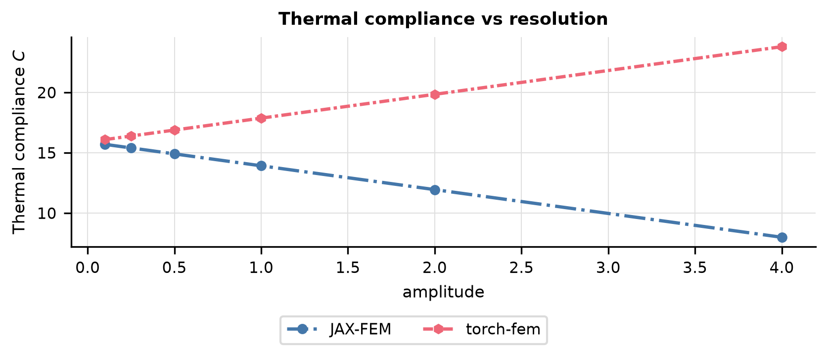
Source Linearity

Thermal compliance \(C\) vs source amplitude at fixed mesh; compares solvers on log-log axes.

Settings

Sweeps amplitude ∈ {0.1, 0.25, 0.5, 1.0, 2.0, 4.0}

{
  "ic": {
    "name": "gaussian_source"
  },
  "physics": {
    "nx": 16,
    "ny": 8,
    "nz": 1,
    "Lx": 2.0,
    "Ly": 1.0,
    "Lz": 1.0,
    "rho_0": 0.5,
    "ic_field": "source",
    "amplitude": 0.1
  },
  "sweep": {
    "key": "amplitude",
    "values": [
      0.1,
      0.25,
      0.5,
      1.0,
      2.0,
      4.0
    ]
  }
}

Solver ranking

Solver	Mean rel. error
deal.II	1.74e-08
FEniCS	1.74e-08
Firedrake	1.74e-08
JAX-FEM	1.74e-08
torch-fem	1.74e-08

Ranked by mean relative error against the reference solution (lower is more accurate).

Cost

What does it cost? Wall-clock scaling of the forward and VJP passes with problem size \(N\) and the number of integration steps. Timings come from dedicated runners with no concurrent workloads; see the reliability note at the top of the page before reading absolute numbers.

Settings

Spatial Cost

Sweeps nx ∈ {16, 32, 64, 128, 256, 512, 1024}

{
  "physics": {
    "Lx": 2.0,
    "Ly": 1.0,
    "Lz": 1.0,
    "Q_total": 1.0,
    "rho_0": 0.5,
    "steps": 1,
    "nx": 16
  },
  "cost": {
    "n_trials": 3
  },
  "sweep": {
    "key": "nx",
    "values": [
      16,
      32,
      64,
      128,
      256,
      512,
      1024
    ]
  }
}

Temporal Cost

Sweeps steps ∈ {1}

{
  "physics": {
    "Lx": 2.0,
    "Ly": 1.0,
    "Lz": 1.0,
    "Q_total": 1.0,
    "rho_0": 0.5,
    "nx": 64,
    "steps": 1
  },
  "cost": {
    "n_trials": 3
  },
  "sweep": {
    "key": "steps",
    "values": [
      1
    ]
  }
}

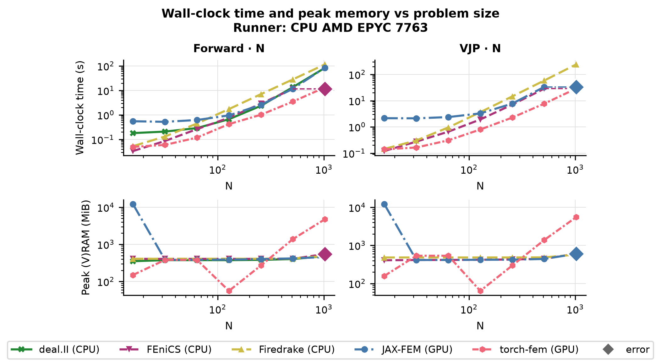
Solver ranking

Solver	Forward time	VJP time
FEniCS	11.7 s @ N=512	28.6 s @ N=512
torch-fem	13.3 s @ N=1024	29 s @ N=1024
deal.II	83.7 s @ N=1024	—
JAX-FEM	84.7 s @ N=1024	33.5 s @ N=512
Firedrake	116 s @ N=1024	242 s @ N=1024

Forward and VJP (backward) wall-clock time, each shown at the largest problem size N the solver completed for that pass; ranked by forward time (faster is better). Forward-only solvers have no VJP entry. See the reliability note above before comparing across devices.

Gradient

Is the gradient right? Gradient benchmarks compare each solver’s AD/adjoint gradient against a finite-difference ground truth. We report magnitude error (relative \(L^2\)) and direction agreement (cosine similarity) across parameter, resolution, and horizon sweeps. The horizon sweep in particular exposes how gradients degrade as the rollout lengthens.

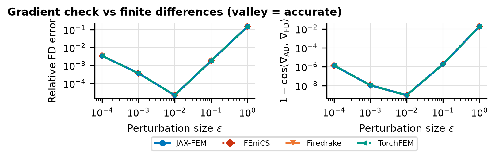
Finite-Difference Check

FD gradient error vs step size \(\varepsilon\) (U-curves), AD/FD direction cosine, and gradient magnitude field panels.

Settings

{
  "ic": {
    "name": "random",
    "seed": 0
  },
  "physics": {
    "nx": 8,
    "ny": 4,
    "nz": 1,
    "Lx": 2.0,
    "Ly": 1.0,
    "Lz": 1.0,
    "Q_total": 1.0
  },
  "fd": {
    "eps_values": [
      1.0,
      0.1,
      0.01,
      0.001,
      0.0001
    ],
    "n_dirs": 6
  }
}

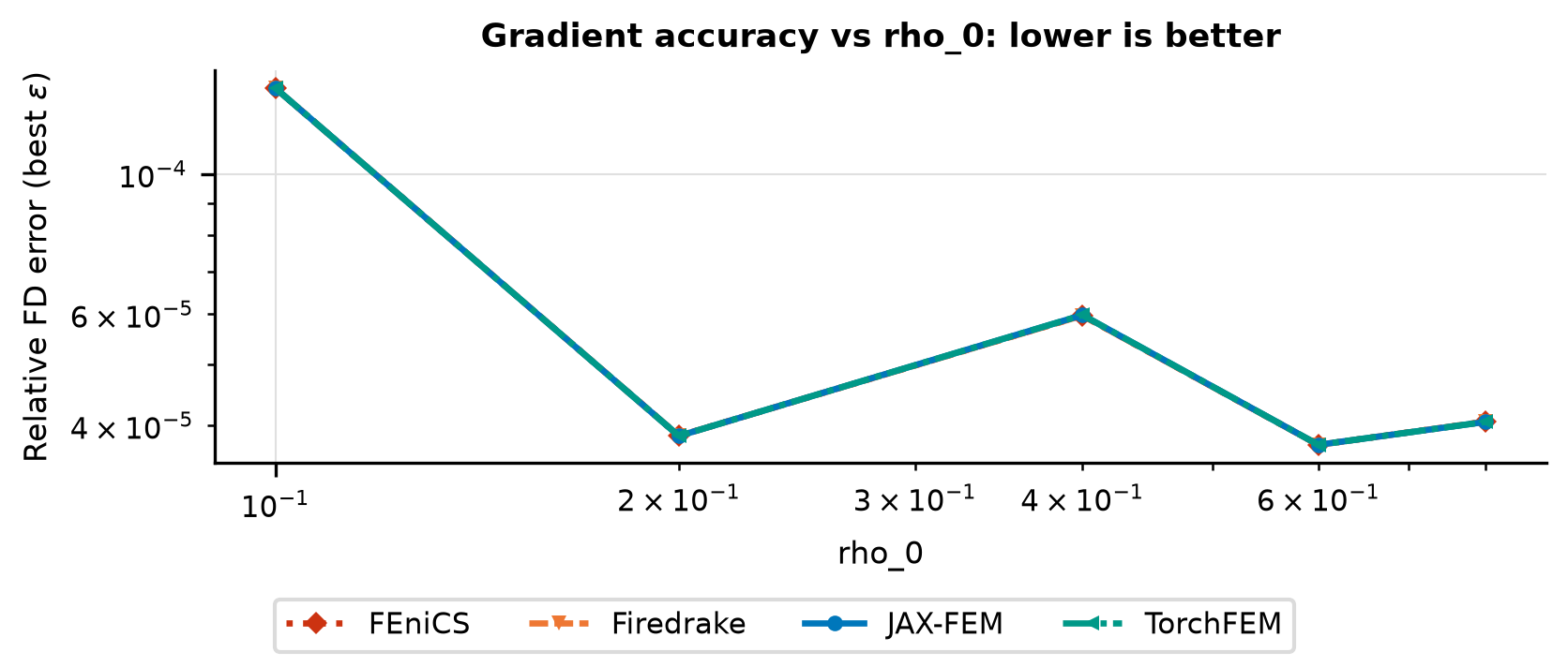
Parameter Sweep

Gradient norm, best-\(\varepsilon\) FD error, AD/FD direction cosine, and U-curves vs element density \(\rho_0\).

Settings

Sweeps rho_0 ∈ {0.1, 0.2, 0.4, 0.6, 0.8}

{
  "ic": {
    "name": "uniform",
    "seed": 0
  },
  "physics": {
    "nx": 8,
    "ny": 4,
    "nz": 1,
    "Lx": 2.0,
    "Ly": 1.0,
    "Lz": 1.0,
    "Q_total": 1.0,
    "rho_0": 0.1
  },
  "fd": {
    "eps_values": [
      1.0,
      0.1,
      0.01,
      0.001,
      0.0001
    ],
    "n_dirs": 6
  },
  "sweep": {
    "key": "rho_0",
    "values": [
      0.1,
      0.2,
      0.4,
      0.6,
      0.8
    ]
  }
}

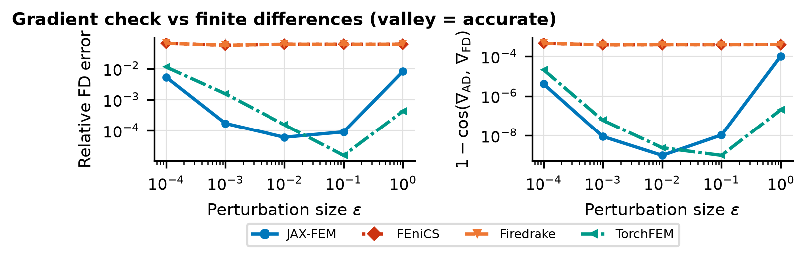
Source Fd Check

FD gradient error vs \(\varepsilon\), AD/FD direction cosine, and gradient field panels for d(identification_error)/d(source).

Settings

{
  "ic": {
    "name": "gaussian_source"
  },
  "ic_key": "source",
  "output_key": "identification_error",
  "physics": {
    "nx": 8,
    "ny": 4,
    "nz": 1,
    "Lx": 2.0,
    "Ly": 1.0,
    "Lz": 1.0,
    "rho_0": 0.5,
    "target_from_two_gaussians": true,
    "ic_field": "source"
  },
  "fd": {
    "eps_values": [
      1.0,
      0.1,
      0.01,
      0.001,
      0.0001
    ],
    "n_dirs": 6
  }
}

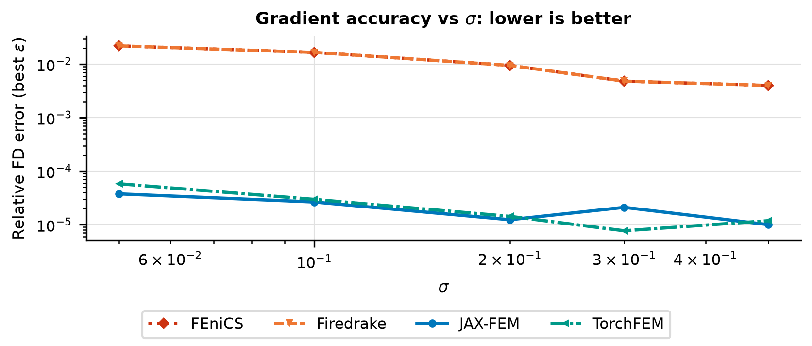
Source Width Sweep

Gradient norm, best-\(\varepsilon\) FD error, AD/FD direction cosine, and U-curves vs source width \(\sigma\).

Settings

Sweeps sigma ∈ {0.05, 0.1, 0.2, 0.3, 0.5}

{
  "ic": {
    "name": "gaussian_source"
  },
  "ic_key": "source",
  "output_key": "identification_error",
  "physics": {
    "nx": 16,
    "ny": 8,
    "nz": 1,
    "rho_0": 0.5,
    "target_from_two_gaussians": true,
    "ic_field": "source"
  },
  "fd": {
    "eps_values": [
      0.1,
      0.01,
      0.001,
      0.0001
    ],
    "n_dirs": 4
  },
  "sweep": {
    "key": "sigma",
    "values": [
      0.05,
      0.1,
      0.2,
      0.3,
      0.5
    ],
    "ic_sweep": true
  }
}

Solver ranking

Solver	Best-ε FD error	1 − cosine
FEniCS	1.83e-05	2.21e-10
Firedrake	1.83e-05	2.21e-10
JAX-FEM	1.83e-05	2.21e-10
torch-fem	1.83e-05	2.21e-10

Ranked by the best-ε finite-difference error of the gradient (lower is more trustworthy); direction cosine near 1 confirms the gradient points the right way.

Optimization

Can you optimize through it? End-to-end optimization benchmarks run a gradient-based optimizer using each solver’s own gradients: recovery of initial conditions or physical parameters, topology optimization, and drag minimization. This is the ultimate test, since a gradient can pass the finite-difference check yet still fail to drive a full optimization loop.

Conductivity Recovery Bfgs

Optimisation traces (loss vs iteration) and recovered conductivity fields vs the two-Gaussian ground truth, using L-BFGS.

Settings

{
  "ic": {
    "name": "uniform",
    "seed": 0
  },
  "physics": {
    "nx": 16,
    "ny": 8,
    "nz": 1,
    "Lx": 2.0,
    "Ly": 1.0,
    "Lz": 1.0,
    "rho_0": 0.5,
    "Q_total": 1.0,
    "compliance_key": "identification_error",
    "penalty_weight": 0.0,
    "x_min": 0.001,
    "snap_interval": 10,
    "target_rho_from_two_gaussians": true
  },
  "optim": {
    "max_iters": 200,
    "patience": 30
  },
  "optimizer": "bfgs"
}

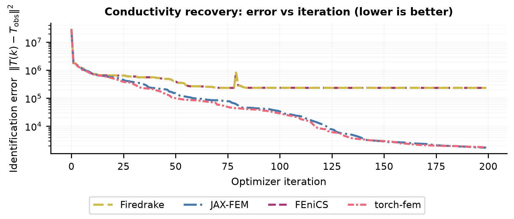
Solver ranking

Solver	Final error	Converged
JAX-FEM	1.72e+03	no
torch-fem	1.75e+03	no
FEniCS	2.33e+05	no
Firedrake	2.33e+05	no

Ranked by the final objective reached within the iteration budget (lower is better).