← Tesseract Blog

2026-10-25 · @dionhaefner

Fast, GPU-native differentiable physics and beyond with Tesseract

Tesseract lets you put a differentiable physics simulation inside a JAX or PyTorch training loop. Paired with Tesseract-JAX and Tesseract-Torch, the simulator runs in its own process or container, while the training loop treats it like any other differentiable function. Until now, every GPU array passed into or out of a Tesseract was copied through host memory, which for large arrays can take longer than the computation itself. The new GPU transport removes this detour, so arrays stay on the GPU the whole way. This post shows what that unlocks on a real application, how to turn it on, and what happens under the hood when passing GPU memory up and down the call stack (and over HTTP between processes).

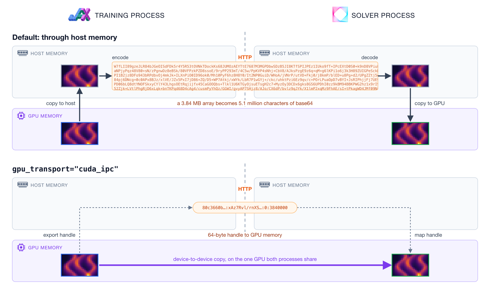
Two ways a GPU array travels to a Tesseract in another process. Through the host, every byte leaves the GPU and is encoded as text. With cuda_ipc, only a handle is sent via HTTP, and outputs are returned the same way.

The problem

It all started with the winning entry of our first hackathon, Multi-Agent-DPC by Pietro Zanotta, Dibakar Roy, and Honghui Zheng, which later grew into the ICML 2026 paper CINOC. It learns an optimal control policy for a swarm of mobile heaters that shape the temperature along a rod. The policy is a small neural network that decides how hard each heater heats or cools and where it moves, and it is trained by backpropagating through 300 steps of a differentiable PDE solver. The team wrapped the solver as a Tesseract and called it from their JAX training loop through Tesseract-JAX.

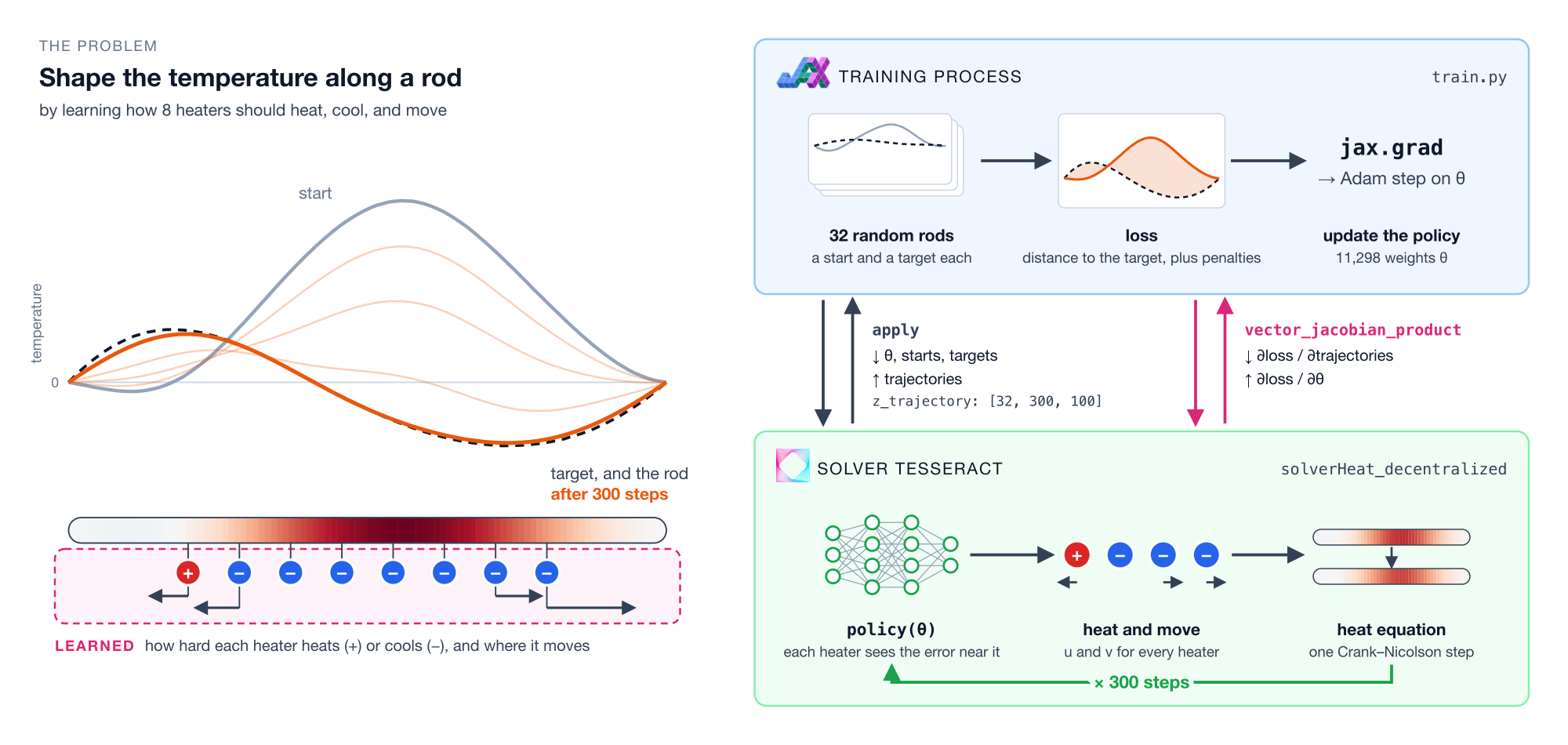
Left, one Multi-Agent-DPC task, solved with the team’s trained policy. The policy decides how each of the eight heaters heats, cools, and moves. Over 300 steps it drives the rod from its starting temperature (gray) onto the target (dashed). Right, one training step. The training loop samples 32 rods and calls the solver Tesseract twice, through apply for the trajectories and through vector_jacobian_product for the gradient with respect to the policy’s weights.

It worked but was too slow to train with, so the team’s training script ended up calling the solver directly with the Tesseract path switched off. They published a branch that reproduces the slowdown, and over the following months we used it as a benchmark to make Tesseract faster for differentiable physics applications, one release at a time.

A deeper problem was the data communication overhead. Each array left the GPU, was encoded as text into a JSON body, sent over HTTP, and was decoded and copied back onto the GPU on the other side, once for the forward pass and once for the gradient. Through that path, running the solver on the GPU gained so little that it was faster to run it on CPU instead.

With the new GPU transport capabilities in Tesseract Core (v1.15.0), Tesseract-JAX (v0.5.0), and Tesseract-Torch (v0.2.0), arrays now stay where they are. Only a 64-byte handle is sent across the process boundary, and the data moves only within the memory of the GPU, which is shared by both processes. Together with better batching support and a cache for the solver’s forward pass, this brings Multi-Agent-DPC’s training step within 20% of importing the solver directly. For the much larger arrays common in 3D simulation, transport is now two orders of magnitude faster than the trip through host memory.

Why not just import the solver?

If you can import a component, import it. The Multi-Agent-DPC team came to the same conclusion, and the code for CINOC imports its solvers directly.

But often you can’t. Many entries to this year’s Tesseract Hackathon were built around components that did not want to be imported into Python directly. δSnowSac trains a PyTorch network through NOAA’s Fortran streamflow models, PRISMO takes one JAX gradient through a Julia semiconductor solver and a FEniCS optics solver, and Differentiable Silicon dispatches to a proprietary TCAD binary over SSH. Mosaic puts solvers from deal.II and OpenFOAM to JAX-FEM and XLB behind the same Tesseract interface, each with its own dependencies. Tesseract puts such a component in its own process or container and still allows it to participate in differentiable pipelines. See also When to use Tesseract.

A faster, GPU-native Multi-Agent-DPC

Let’s turn on GPU transport for the Multi-Agent-DPC training loss, with the solver served from the team’s tesseract_api.py. Passing gpu_transport="cuda_ipc" to the Tesseract constructor is all you need (see also Keep GPU arrays on the device with cuda_ipc), and Tesseract-JAX picks it up from there:

import os

# NEW: two JAX processes now share one GPU, so neither should claim 75% of it at startup.
os.environ["XLA_PYTHON_CLIENT_PREALLOCATE"] = "false"

import jax
from jax.flatten_util import ravel_pytree
from tesseract_core import Tesseract
from tesseract_jax import apply_tesseract

solver = Tesseract.from_source(
    "tesseracts/solverHeat_decentralized/tesseract_api.py",
    gpu_transport="cuda_ipc",  # NEW: pass GPU arrays by handle (2)
)


def loss(params, z_init, xi_init, z_target):
    inputs = {
        "z_init": z_init,
        "xi_init": xi_init,
        "z_target": z_target,
        "flat_params": ravel_pytree(params)[0],
    }
    # NEW: one call for the whole batch instead of one per rollout (1)
    traj = apply_tesseract(solver, inputs, vmap_method="broadcast_all")
    return tracking_error(traj["z_trajectory"], z_target) + penalties(traj)


def batch_loss(params, z_init, xi_init, z_target):
    losses = jax.vmap(loss, in_axes=(None, 0, 0, 0))(params, z_init, xi_init, z_target)
    return losses.mean()


with solver:
    grads = jax.jit(jax.grad(batch_loss))(params, z_init, xi_init, z_target)

This deviates from the original script in two ways:

1. apply_tesseract(..., vmap_method="broadcast_all") sends the whole batch of rollouts to the Tesseract as one call, which the solver supports by accepting an optional leading batch dimension.

2. Tesseract.from_source(..., gpu_transport="cuda_ipc") enables the GPU transport for a source-built Tesseract (a containerized Tesseract works the same way through Tesseract.from_image(..., gpus=["all"], gpu_transport="cuda_ipc")).

For applications that use torch instead of JAX, Tesseract-Torch works in exactly the same way with an identical apply_tesseract function.

Turns out it’s pretty good

Here is one training step of Multi-Agent-DPC, that is, a batch of 32 rollouts forwards and backwards, as it went from the team’s setup to the GPU path (benchmark script):

Setup	Time per training step
The original setup, on current Tesseract releases	1.5 s
Batched, solver on the GPU, arrays through host memory	261 ms
Same, with cuda_ipc	209 ms
Same, with the solver’s VJP cache	127 ms
Solver imported directly, one process (baseline)	106 ms

The GPU transport removes the trip through host memory, which saves about 50 ms per step. The VJP cache, an experimental option in Tesseract’s JAX recipe, saves another 80 ms by keeping the residuals of the forward pass, so the gradient call doesn’t rerun all 300 steps. What remains, about 20 ms per step, is mostly the fixed cost of two HTTP requests and the handle exchange.

A Multi-Agent-DPC call moves about 4.8 MB in and out combined, which is modest. How much the transport matters depends mostly on how many bytes are sent across the boundary. The figure below isolates this with a Tesseract that only doubles its input.

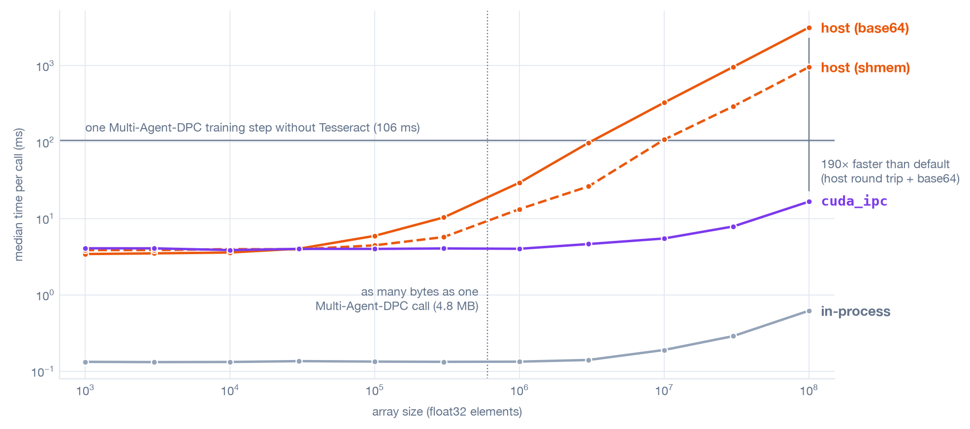
Median time of one jitted apply_tesseract call to a Tesseract that doubles a float32 vector, on an NVIDIA A100 GPU. host (base64) is Tesseract’s default host path. host (shmem) also copies through host memory, but exchanges arrays as binary files on /dev/shm (the json+binref format) instead of base64 text. For scale, the horizontal line marks one Multi-Agent-DPC training step with the solver imported directly, and the dotted line a call that moves as many bytes as one Multi-Agent-DPC call (2.4 MB each way). The benchmark script reproduces the figure.

Below about 100 kB per call, the trip through host memory is the fastest option, because the GPU transport has a slightly higher fixed cost. Above that, the host path grows linearly by about 8 ms per megabyte, spent on copies and text encoding on the CPU, while cuda_ipc stays nearly flat. At 100 million values, or 400 MB, the GPU transport is 190 times faster than Tesseract’s default host path, and still almost 60 times faster than exchanging raw binary data via shared memory.

Beyond Multi-Agent-DPC

So far, using Tesseract hasn’t really been feasible for GPU-based training through a differentiable solver. The new GPU transport changes that, making it practical for scenarios such as:

• Solver in the loop. A network learns to correct a coarse simulation, and its loss is computed after unrolling the solver + network system for many steps (Um et al., 2020; Kochkov et al., 2021).

• Learned closures. A network supplies a term the simulator can’t compute efficiently, such as subgrid-scale stresses in turbulence, and is trained through the simulation (List et al., 2022; NeuralGCM for weather and climate). Idealized example: Our learned closure demo does this for a viscosity model in Burgers’ equation.

• Control and reinforcement learning. A network is learning to interact with a physical system by training against a differentiable simulator (Holl et al., 2020), as in Multi-Agent-DPC, which builds on differentiable predictive control.

• Served surrogates. A trained surrogate runs as a service on the GPU, and an optimizer or pipeline calls it over and over.

In all of these, the network and the solver both run on the GPU, and training alternates between them thousands of times. Most move far bigger arrays than Multi-Agent-DPC. Sending a single 256³ float32 field (16.8 million values) through the host to a Tesseract and getting one back takes over half a second. With the new GPU transport, it takes about 6 ms.

How the gradient flows up and down the stack

You don’t need to know any of this to use the GPU transport, but to us, how it works is the most remarkable part of the story. Specifically, a single gradient call drops out of compiled XLA code into C++, goes back into the Python interpreter, crosses HTTP into another process, descends into that process’s own XLA, and returns the same way, while the arrays never leave the GPU! (Most of that path is specific to Tesseract-JAX. Tesseract-Torch reaches the same place without a C++ bridge, for reasons we come back to at the end.)

Take these five lines, a stripped-down version of the training loss above:

def loss(theta):
    traj = apply_tesseract(solver, {"theta": theta})["trajectory"]
    return jnp.mean((traj - target) ** 2)

with Tesseract.from_source("./tesseract_api.py") as solver:
    grads = jax.jit(jax.grad(loss))(theta)

When jax.grad runs, JAX asks Tesseract-JAX for a primal and a vector-Jacobian product (VJP). Tesseract-JAX turns this into two requests to the solver, one to apply for the trajectory and one to vector_jacobian_product for the gradient. Here is how the gradient with respect to the trajectory, 3.84 MB of float32 for a batch of 32 rollouts, is represented in the body of the second request:

Through host memory

{
  "object_type": "array",
  "shape": [32, 300, 100],
  "dtype": "float32",
  "data": {
    "buffer": "slPUPa5mfD5CBcs9OirIvgsQiz5TIAk+uPMkvv2EMj5I/t89C7e0PXWzPRUWPdbiFD2WZBI9SKoPPeagDD1KNAk96E8FPZzfAD3UoPc8KCPsPKgq3zwIo9A8EIHAPEDDrjyocps8AKOGPFDlYDyAFDI8sDYBPEB9nTsAXtk6AMzHukBHmruQwwC8gEwzvGA3ZLwIg4m8AKOfvABJtLzwSce8CIPYvNjZ57w4PPW8PFAAvXYCBb2otwi9OHYLvcdHDb3AOA69C1gOvaO2Db0gZwy9VH0KvdANCL1xLQW95PABvWDY/LyIZPW8BKntvLTE5bz40d28EObVvJAQzrwwW8a8yMm+vGBat7xYBbC8AL6ovBBzobyoD5q8CHySvGCeirxgXIK84DdzvCCIYLwgfEy8AO42vIC/H7yg3Aa8AHjYuwDBn7uAZUe7AA6SugDgazoAzkM7QEOoO0AF8DsAShw8YKZAPIDEZDywKIQ8IH6VPNA8pjxwQrY8cHHFPOCx0zxA8eA8qCPtPMBD+DwoKQE9/KoFPWytCT3YOA09blcQPcwUEz14fRU9Up4XPS+EGT1uOxs95gwcPXezFj3IfxU9...",
    "encoding": "base64"
  }
}

With cuda_ipc

{
  "object_type": "array",
  "shape": [32, 300, 100],
  "dtype": "float32",
  "data": {
    "buffer": "80c3660b-f7b0-48f9-8ad6-7f36c1e7e9bf:xAz7Rvl/rnXSpn869f++dNC9NWxplFo3qLs+qce5gyNA1eMWkRWGatgyGZfLq4e001iiEs3oW+hxjxR7Q+f2cg==:0:3840000",
    "encoding": "cuda_ipc"
  }
}

The base64 buffer goes on for another 5.1 million characters, while the cuda_ipc buffer is complete. It contains the GPU’s UUID, a 64-byte CUDA IPC handle that another process on the same machine can use to map the same allocation, and the position of the array within that allocation. Shapes and dtypes stay in the JSON payload, so the server still validates every request against its schema.

Getting from those five lines to that request and back takes the path below, spanning Python, C++, CUDA, and HTTP across process boundaries.

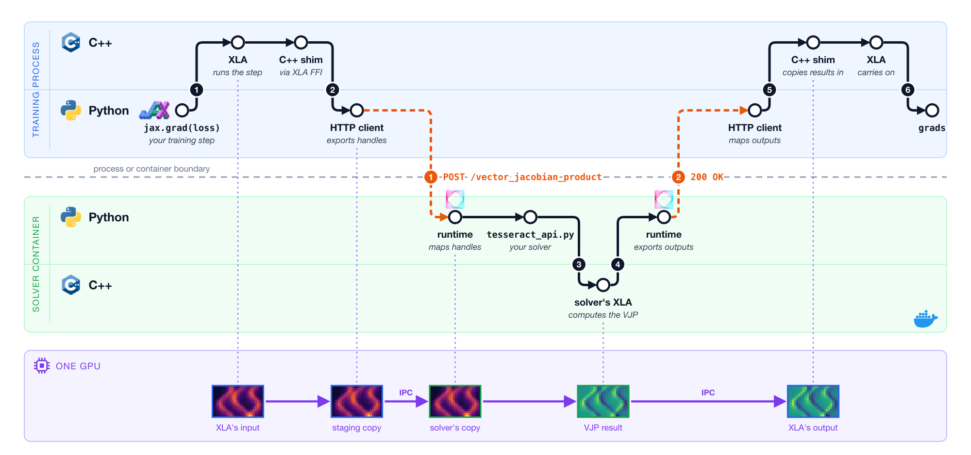
One VJP call, left to right. It switches between Python and C++ six times and crosses into the solver’s process twice, while the array data never leaves the memory of the shared GPU.

The C++ bridge of Tesseract-JAX is needed because under jit, XLA needs to know how to run the primitive without copying data. On the CPU everything runs as a host callback into Python which receive NumPy arrays, so XLA copies every input off the device before Python sees it, and no code downstream could undo that. JAX has no Python-level API for handing GPU buffers out of a compiled program, so the fix had to be native. On CUDA, Tesseract-JAX now lowers the primitive to an XLA FFI custom call into a small C++ shim, which receives raw device pointers from XLA and waits for XLA’s stream so the inputs are ready. The shim loads the CUDA runtime only when first used, so the same wheel installs and runs on machines without a GPU.

The next step is the craziest one: While XLA is in the middle of running a compiled program, the shim (called from one of XLA’s threads) takes Python’s global interpreter lock and calls back into the Python interpreter. Each call site keeps track of an integer token, baked into the compiled program as an FFI attribute, which the shim uses to look up the Python closure for that particular call. The closure receives the device pointers as minimal objects that expose __cuda_array_interface__, passes them to the Tesseract’s Python client, and waits for the solver to answer. Only then does control return to C++, and from there to XLA.

Another complication is that XLA allocates GPU memory through CUDA’s virtual memory management API, which does not support legacy CUDA IPC handles. So the client first copies each array into a buffer it can export (and reuses those buffers from call to call). For PyTorch, Tesseract-Torch needs none of this. Its tensors already expose their device pointers to Python, so Tesseract-Torch calls the same client without native code, and with PyTorch’s default allocator also without the extra copy.

Most mistakes in code like this return wrong numbers or quietly fall back to the host instead of crashing, so there was a lot of stress-testing involved. We had to set up GPU tests to reject any pointer that isn’t in GPU memory, so an accidental trip through the host fails loudly. And a Tesseract created with gpu_transport="cuda_ipc" checks before its first call that the transport works between the two processes, and raises with the reason instead of falling back to the host. The troubleshooting section of the how-to covers more common failure modes, such as JAX itself running on the CPU.

What’s next

Today, Tesseract’s GPU transport is built on CUDA IPC, which works great and is fast, but it means the caller and the Tesseract must have direct memory access to the same GPU. However, GPU transport selection is already fully generic in Tesseract, so adding support for other transport mechanisms can be done without changing the user experience or the core logic of Tesseract.

A logical next step is supporting communication across multiple machines. An experimental nixl transport built on NVIDIA’s NIXL transfer library moves GPU memory through CUDA IPC on the same host and through UCX between hosts. This includes RDMA over NVLink or Infiniband (reading directly from and to device memory) where the hardware supports it. Triggering a request still works with a short descriptor instead of the full array bytes, so with GPUDirect RDMA, a training loop on one machine could call a GPU solver on another without the arrays passing through host memory on either side.

Try it

The GPU transport has a few requirements on both sides of the boundary, from the GPU and CUDA setup to a Tesseract that can consume and return GPU arrays. Start with the GPU transport how-to, which walks through them and covers every way to serve and call a Tesseract with the transport. Once those are in place, enabling it takes one extra argument:

Tesseract-JAX

from tesseract_core import Tesseract
from tesseract_jax import apply_tesseract

solver = Tesseract.from_image("my-solver", gpus=["all"], gpu_transport="cuda_ipc")

with solver:
    outputs = apply_tesseract(solver, inputs)  # GPU arrays in and out, no host copies

Tesseract-Torch

from tesseract_core import Tesseract
from tesseract_torch import apply_tesseract

solver = Tesseract.from_image("my-solver", gpus=["all"], gpu_transport="cuda_ipc")

with solver:
    outputs = apply_tesseract(solver, inputs)  # CUDA tensors in and out, no host copies

Python SDK

from tesseract_core import Tesseract

solver = Tesseract.from_image("my-solver", gpus=["all"], gpu_transport="cuda_ipc")

with solver:
    outputs = solver.apply(inputs)  # CuPy, JAX, or PyTorch GPU arrays in, device arrays out

Command line

$ tesseract serve my-solver --gpus all -e TESSERACT_GPU_TRANSPORT=cuda_ipc

Tesseract-JAX and Tesseract-Torch use the transport for a Tesseract created with Tesseract.from_url, as long as it works from the calling process.

From there:

• Tesseract-JAX and Tesseract-Torch are the places to start if your training loop lives in one of those frameworks.

• New to Tesseract? The getting started guide covers building and serving your first Tesseract.

If you have a GPU component that lives in another stack, or a training loop that currently bounces arrays through the CPU, we’d like to hear how the new GPU transport works for you!

---

Discuss this post on the Tesseract Forum

Tesseract is a free, open-source framework for differentiable scientific computing.
Docs · Demos · GitHub