Wrapping Compiled Code (Fortran Example)
Context
Many industries—aerospace, energy, automotive—rely on simulation codes written in compiled languages like Fortran that have been developed and validated over decades. These legacy assets represent significant investment and domain expertise. Tesseract provides a straightforward path to wrap such codes, making them accessible through a modern API while preserving their proven numerical implementations.
This example demonstrates how to wrap a Fortran heat equation solver as a Tesseract using subprocess-based integration. The pattern shown here applies to any compiled executable, whether Fortran, C, C++, or other languages.
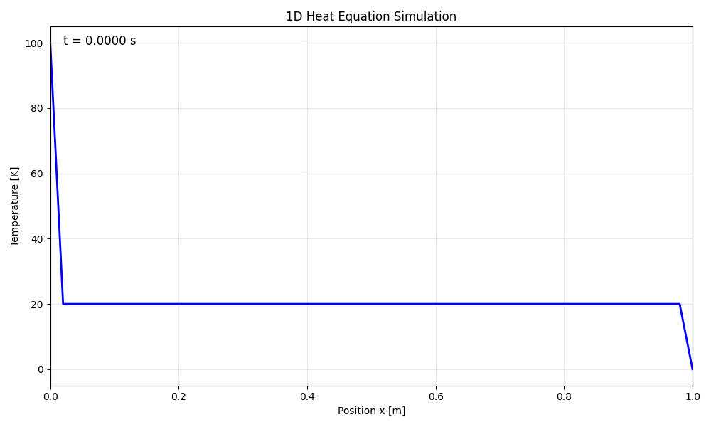
Animation of the 1D heat equation solution showing temperature diffusing from a hot boundary (left, 100K) through an initially cold material toward a cold boundary (right, 0K).
Example Tesseract (examples/fortran_heat)
The Fortran solver
The solver implements a 1D transient heat equation using explicit finite differences:
where \(T(x,t)\) is temperature and \(\alpha\) is thermal diffusivity. The Fortran code reads parameters from a text file and writes results to a binary file:
! 1D Transient Heat Equation Solver
! =================================
! Solves: dT/dt = alpha * d^2T/dx^2
! Method: Explicit finite difference (forward Euler in time, central difference in space)
!
! Usage: heat_solver <input_file> <output_file>
!
! Input file format (text, one parameter per line):
!   n_points <integer>
!   n_steps <integer>
!   alpha <real>
!   length <real>
!   dt <real>
!   t_left <real>
!   t_right <real>
!   initial_temperature <real>
!
! Output file format (binary):
!   n_points (int32)
!   n_steps (int32)
!   x(1:n_points) (float64)
!   T_history(1:n_points, 1:n_steps+1) (float64, column-major)
Input and output schemas
The InputSchema defines the simulation parameters with physical descriptions and validation. Notably, it includes a CFL stability check—the explicit finite difference scheme requires \(r = \alpha \Delta t / \Delta x^2 \leq 0.5\) for numerical stability:
class InputSchema(BaseModel):
    """Input parameters for the 1D transient heat equation solver.

    Solves: dT/dt = alpha * d^2T/dx^2
    with Dirichlet boundary conditions on a domain [0, length].
    """

    n_points: int = Field(
        default=51,
        ge=3,
        le=1001,
        description="Number of spatial grid points. Must be >= 3.",
    )
    n_steps: int = Field(
        default=100,
        ge=1,
        le=10000,
        description="Number of time steps to simulate.",
    )
    alpha: float = Field(
        default=0.01,
        gt=0.0,
        description="Thermal diffusivity [m^2/s]. Material property that characterizes "
        "how quickly heat diffuses through a material.",
    )
    length: float = Field(
        default=1.0,
        gt=0.0,
        description="Domain length [m].",
    )
    dt: float = Field(
        default=0.001,
        gt=0.0,
        description="Time step size [s].",
    )
    t_left: float = Field(
        default=100.0,
        description="Temperature at left boundary (x=0) [K or degC].",
    )
    t_right: float = Field(
        default=0.0,
        description="Temperature at right boundary (x=length) [K or degC].",
    )
    initial_temperature: float = Field(
        default=0.0,
        description="Initial temperature throughout the domain [K or degC].",
    )

    @model_validator(mode="after")
    def check_stability(self) -> Self:
        """Check CFL stability condition for explicit scheme.

        The explicit finite difference scheme is stable only when
        r = alpha * dt / dx^2 <= 0.5 (von Neumann stability analysis).
        """
        dx = self.length / (self.n_points - 1)
        r = self.alpha * self.dt / (dx * dx)
        if r > 0.5:
            raise ValueError(
                f"Stability condition violated: r = alpha*dt/dx^2 = {r:.4f} > 0.5. "
                f"Either reduce dt, reduce alpha, or increase n_points to satisfy "
                f"the CFL condition for the explicit scheme."
            )
        return self
The OutputSchema returns the full temperature history along with convenience fields:
class OutputSchema(BaseModel):
    """Output from the heat equation solver."""

    x: Array[(None,), Float64] = Field(
        description="Spatial coordinates [m]. Shape: (n_points,)",
    )
    temperature: Array[(None, None), Float64] = Field(
        description="Temperature history [K or degC]. Shape: (n_steps+1, n_points). "
        "First row is the initial condition, last row is the final state.",
    )
    final_temperature: Array[(None,), Float64] = Field(
        description="Final temperature profile [K or degC]. Shape: (n_points,)",
    )
    time: Array[(None,), Float64] = Field(
        description="Time values for each saved step [s]. Shape: (n_steps+1,)",
    )
Subprocess integration
The apply function writes input parameters to a temporary file, invokes the compiled Fortran executable, and reads back the binary results. Output from the solver is streamed in real-time to the parent process:
def apply(inputs: InputSchema) -> OutputSchema:
    """Run the Fortran heat equation solver.

    This function:
    1. Writes input parameters to a temporary file
    2. Calls the compiled Fortran executable via subprocess
    3. Reads the binary output file and returns results as arrays
    """
    solver_path = _get_solver_path()

    with TemporaryDirectory() as tmpdir:
        tmpdir_path = Path(tmpdir)
        input_file = tmpdir_path / "input.txt"
        output_file = tmpdir_path / "output.bin"

        # Write input parameters
        _write_input_file(input_file, inputs)

        # Run Fortran solver with real-time output streaming
        process = subprocess.Popen(
            [str(solver_path), str(input_file), str(output_file)],
            stdout=None,  # Inherit stdout - streams to parent process
            stderr=None,  # Inherit stderr - streams to parent process
        )
        returncode = process.wait()

        if returncode != 0:
            raise RuntimeError(f"Fortran solver failed with return code {returncode}.")

        # Read output
        x, T_history = _read_output_file(output_file)

    # Compute time array
    time = np.arange(inputs.n_steps + 1) * inputs.dt

    return OutputSchema(
        x=x,
        temperature=T_history,
        final_temperature=T_history[-1, :],
        time=time,
    )
Build configuration
The tesseract_config.yaml installs gfortran and compiles the solver during image build:
name: "fortran-heat"
version: "1.0.0"
description: |
  1D transient heat equation solver demonstrating Fortran integration.

  This example shows how to wrap legacy Fortran simulation code as a
  Tesseract using subprocess-based integration. The solver uses an
  explicit finite difference scheme to solve the heat equation:

    dT/dt = alpha * d^2T/dx^2

  Industry relevance: thermal analysis of turbine blades, electronics
  cooling, heat treatment processes, and building physics.

build_config:
  base_image: "debian:bookworm-slim"

  # Install Fortran compiler
  extra_packages:
    - gfortran

  # Copy Fortran source into container
  package_data:
    - ["fortran/heat_solver.f90", "fortran/heat_solver.f90"]

  # Compile Fortran code during image build
  custom_build_steps:
    - |
      RUN gfortran -O2 -o /tesseract/fortran/heat_solver /tesseract/fortran/heat_solver.f90
Key points:
extra_packages: Installs the Fortran compiler via apt-getpackage_data: Copies the Fortran source into the containercustom_build_steps: Compiles the code during image build, so the executable is ready at runtime
Results
The solver produces physically meaningful results. Temperature diffuses from the hot left boundary through the material:
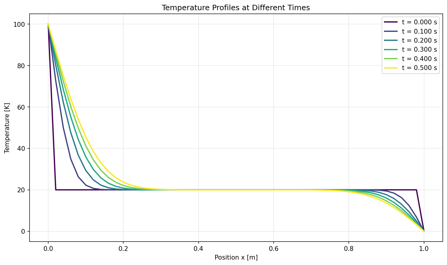
Temperature profiles at different simulation times, showing heat diffusing from the hot boundary (100K at x=0) toward the cold boundary (0K at x=1).
Adapting this pattern
To wrap your own Fortran (or other compiled) code:
Define the I/O protocol: Decide how Python and the executable will exchange data (text files, binary files, stdin/stdout).
Create schemas: Map your solver’s parameters to Pydantic models with validation.
Configure the build: Add compiler installation and compilation steps to
tesseract_config.yaml.Implement
apply(): Write the glue code that marshals data between Python and the executable.
This pattern works for any executable, including MATLAB scripts, Julia programs, or proprietary simulation tools, as long as they can be invoked from the command line.