Performance Trade-offs & Optimization¶

Overview¶

Using Tesseracts adds overhead to your computations through:

Container startup (~2s) — One-time cost when starting a containerized Tesseract.
HTTP communication (~2.5ms locally, up to ~50-100ms+ in cloud setups) — Request/response handling per call.
Data transfer — Moving data between client and server (depends on data size and network bandwidth).
Data serialization — Encoding arrays for transport (depends on data size and encoding format).
Framework overhead (~0.5ms) — Internal machinery, schema processing. Present even in non-containerized mode.

For workloads where computations take seconds or longer, total overhead is typically negligible. See the rules of thumb for guidance on which overhead sources dominate for different workloads.

Note

Tesseract is not a high-performance RPC framework. If your workload requires microsecond latency or millions of calls per second, consider a more traditional RPC framework.

Example scenario: Locally hosted Tesseract¶

Benchmarking scenario¶

The numbers and figures on this page are based on benchmarks run under a specific scenario. This scenario represents a best-case baseline for Tesseract overhead: it minimizes network latency and container virtualization costs, so the numbers isolate framework overhead rather than infrastructure overhead.

Bare-metal Linux Docker (no Docker Desktop virtualization)
Loopback networking (Tesseract running on the same machine as the client)
Local SSD for binref disk I/O
All arrays are float64

Your numbers will differ depending on your setup. In particular:

Docker Desktop (macOS/Windows) adds a virtualization layer, increasing container startup time and HTTP latency, and decreasing raw performance.
Remote Tesseracts make network latency and bandwidth the dominant cost for HTTP mode — compact encodings (base64, binref) matter even more.
Network-attached storage for binref can be significantly slower than local SSD.

Benchmark with representative inputs to understand the trade-offs for your use case.

The right interaction mode depends on your workload¶

Warning

Advice in this section is specific to the benchmarking scenario described above. Your mileage will vary based on your setup and workload.

The following chart shows absolute overhead (in milliseconds) for each interaction mode across a range of array sizes, using a no-op Tesseract that does nothing but decode and encode data:

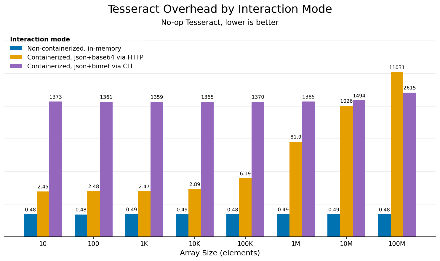
Tesseract overhead by interaction mode — Overhead comparison across interaction modes for different array sizes. Uses a no-op Tesseract that does nothing but decode and encode data, isolating framework overhead.¶

Mode (color)	What it measures	Typical use case
Non-containerized, in-memory (blue)	Direct Python calls via `Tesseract.from_tesseract_api`. Passes data as in-memory Python objects without Docker or HTTP.	Development, tight loops, performance-critical paths
Containerized, json+base64 via HTTP (orange)	Full Docker + HTTP stack, served via HTTP (e.g. `tesseract serve`). Includes serialization and network transfer.	Production, CI/CD, multi-language environments
Containerized, json+binref via CLI (purple)	CLI invocation via `tesseract run`. Includes container startup and disk I/O, but avoids transferring data over the network.	Shell scripts, one-off runs, pipelines with large data

The guidance chart below puts these numbers in context by showing overhead as a percentage of computation time, for three representative I/O sizes (dotted = 1kB, dashed = 1MB, solid = 1GB). For small data, fixed costs (HTTP roundtrip, container startup) dominate. For large data, transfer and serialization take over.

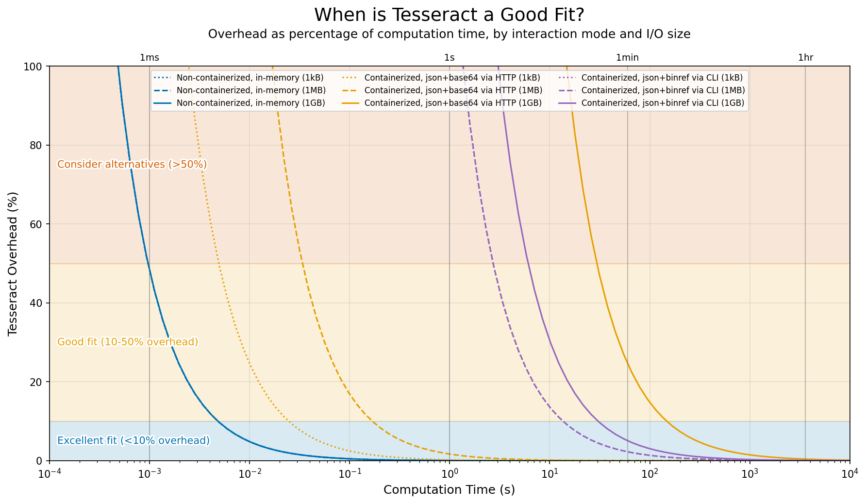
Tesseract overhead guidance chart — Overhead as percentage of computation time, depending on interaction mode and I/O data size, for the benchmark scenario (local Tesseract with fast network and disk). Some lines overlap where modes have similar performance characteristics: non-containerized usage across all data sizes, and CLI usage for all but the largest data sizes.¶

Rules of thumb by use case¶

Warning

Advice in this section is specific to the benchmarking scenario described above. Your mileage will vary based on your setup and workload.

Scenario	Recommendation
Second-scale workloads on medium-size data	The sweet spot for containerized HTTP execution, with low overhead benefitting from most Tesseract features.
Development and debugging	Use non-containerized execution or tesseract-runtime serve for fast iteration, then switch to containerized HTTP for final testing.
Cheap operations on small data via HTTP	HTTP overhead (~2.5ms) can dominate when computation is fast. Batch multiple inputs into a single request.
Tight loops on in-memory data	Consider non-containerized execution to bypass all network/container overhead. At ~0.5ms per call, you can run thousands of iterations per second. Requires all dependencies to be available in the same local Python environment.
Shell scripts and one-off runs	CLI is convenient but has ~2s overhead per invocation from container startup. For multiple calls, keep a container running.
Long-running operations on large datasets	Use CLI with `json+binref` encoding. The ~2s container overhead is negligible for multi-minute runs, and binref allows large arrays to be passed between Tesseracts without expensive copies.
Cheap operations on huge datasets	Serialization and transfer will dominate. Try partitioning your workload so each Tesseract call does more compute per byte of I/O, or use binref to avoid redundant data copies between pipeline stages.

Optimizing performance¶

1. Choose the right encoding format¶

Encoding format affects both serialization time and the volume of data transferred. A 10M-element float64 array is ~76MB as raw binary, ~100MB as base64, and ~230-760MB as JSON. If I/O is slow, data transfer dominates over serialization, and choosing a compact format is the most effective optimization.

In short: use base64 (default) for HTTP transport, binref for large arrays or disk-based pipelines, and json only when you need human-readable output. See Array Encodings for format details and usage examples.

2. Batch small operations¶

If you have many small operations, batch them into a single request:

# ❌ Avoid: Many small calls
for item in items:
    result = tesseract.apply({"data": item})

# ✅ Prefer: Batch into one call
results = tesseract.apply({"data": np.stack(items)})

Note that your Tesseract’s apply function must be written to accept batched inputs (e.g., arrays with a leading batch axis) for this to work.

3. Reuse Tesseract instances¶

Container startup is expensive. Reuse instances across calls:

# Good - reuse the context
with Tesseract.from_image("my-tesseract") as tesseract:
    for batch in batches:
        result = tesseract.apply(batch)

# Bad - new container per call
for batch in batches:
    with Tesseract.from_image("my-tesseract") as tesseract:
        result = tesseract.apply(batch)

If you’re running a script multiple times against the same Tesseract, consider keeping a container running and connecting via Tesseract.from_url():

# Start once: tesseract serve my-tesseract
tesseract = Tesseract.from_url("http://localhost:8100")
result = tesseract.apply(inputs)

4. Profile to find bottlenecks¶

Enable profiling to see where time is spent:

# Via CLI
tesseract run myimage apply '{"inputs": {...}}' --profiling

Or via the Python SDK:

tess = Tesseract.from_tesseract_api(
    "/path/to/tesseract_api.py",
    runtime_config={"profiling": True}
)

See Profiling in the debugging guide for more usage examples and how to interpret the output.