2025-08-03 · @jacanchaplais

Playing Catch With Newton: a Beginner’s Guide to Tesseracts¶

This post originally appeared on Pasteur Labs Insights.

Introduction¶

This tutorial introduces the Tesseract ecosystem through a physics-based example. We’ll build a Tesseract from scratch that containerizes a computational tool and implements derivative endpoints for use in differentiable pipelines.

This beginner’s guide will teach you how to write a custom Tesseract to distribute a computational tool. We assume basic differential calculus knowledge and Python familiarity (including NumPy-style array operations). No prior Tesseract ecosystem experience is required.

The physics: Projectile motion¶

Researchers regularly use fantastic software tools — physics simulators, machine learning models, meshers, and more. But these tools often present installation and configuration barriers for new users. With Tesseracts, you can wrap any tool so it’s installable locally via a single command or accessible remotely, all sharing a uniform JSON interface.

To see how this works, let’s start with a simple physics example: projectile motion.

Newton’s challenge¶

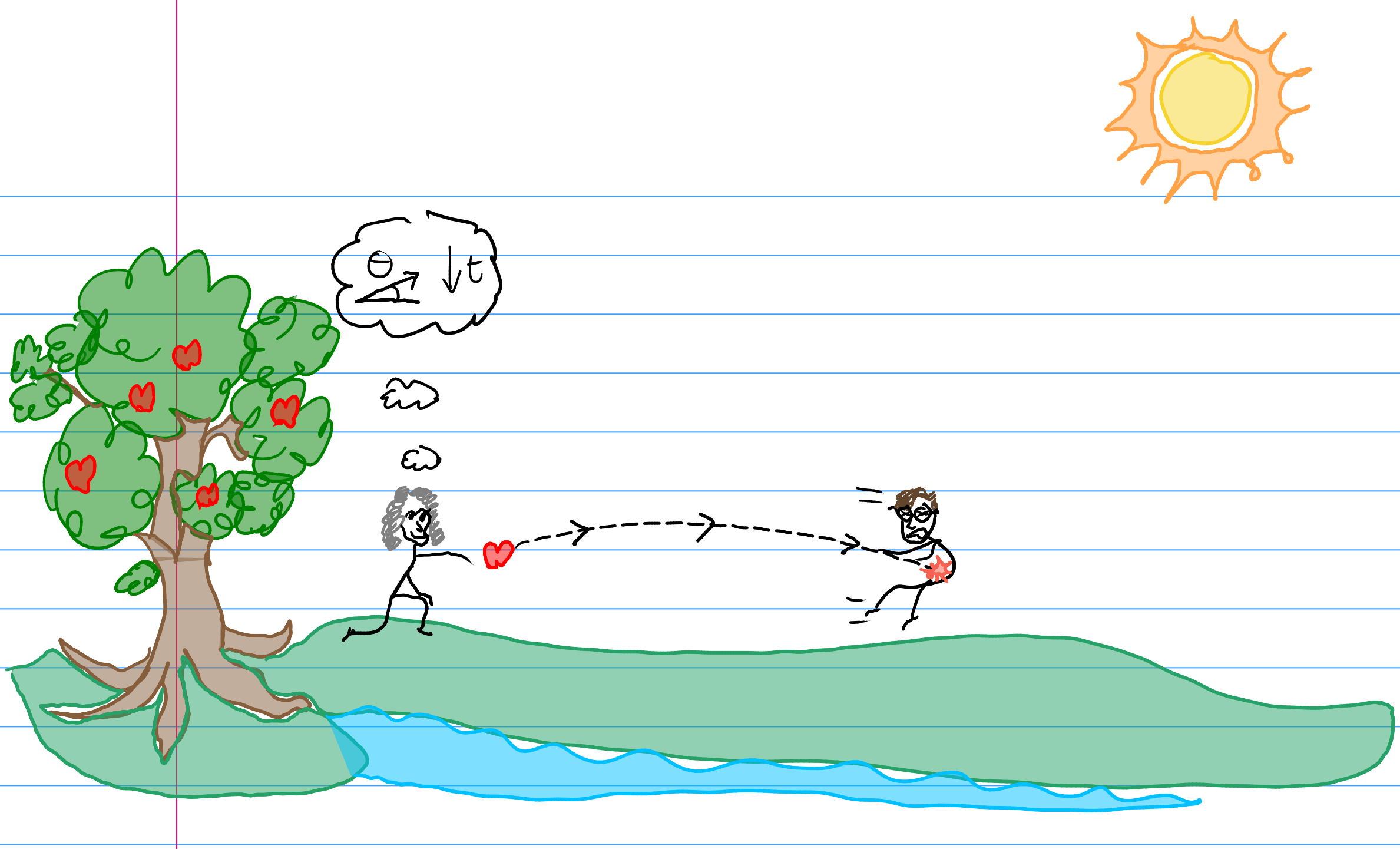
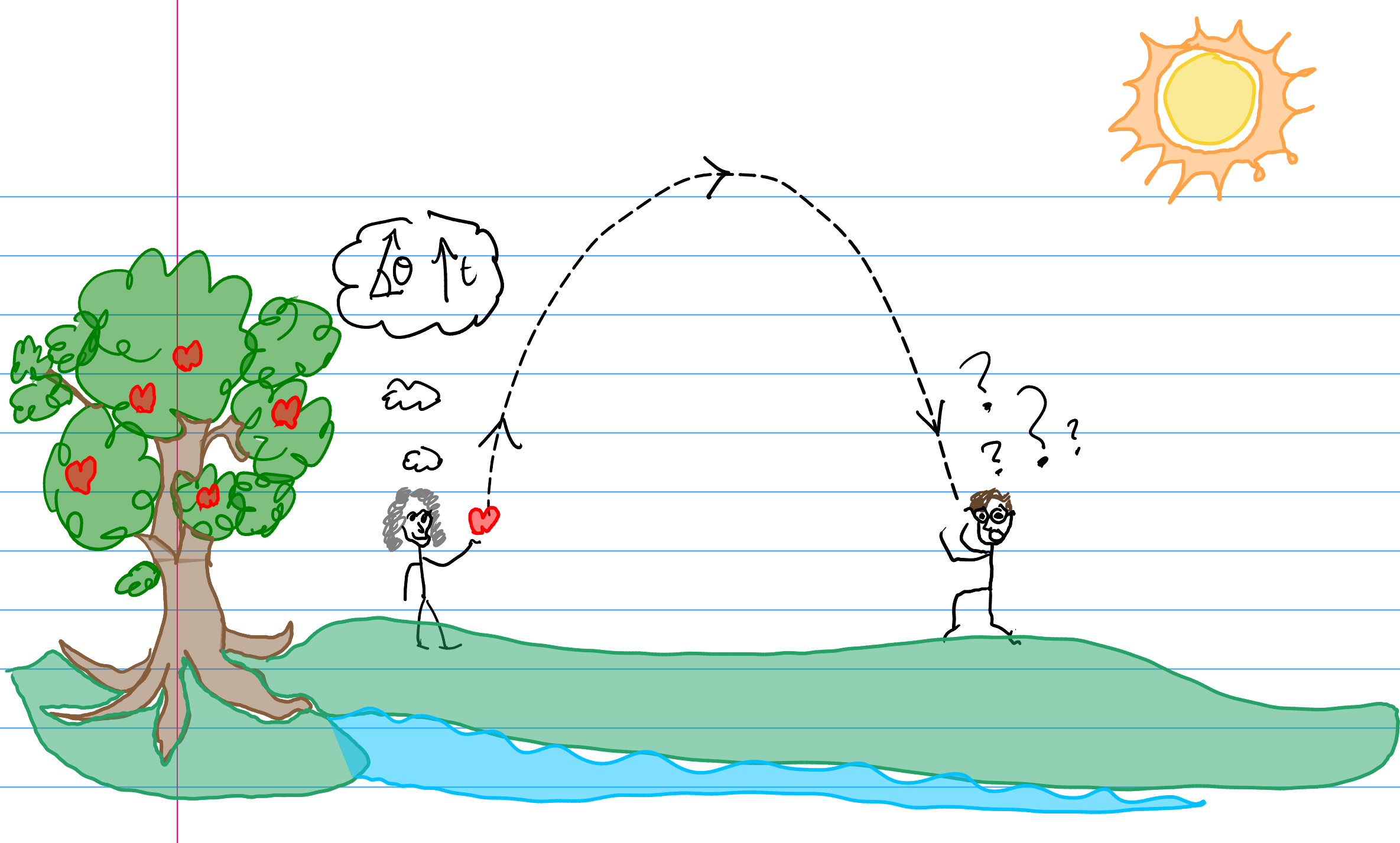
Newton at a low angle — Newton throws a ball at a low angle.

Imagine you’re playing catch with Isaac Newton. He throws a ball from a fixed distance away, and it arrives after a certain flight time. Newton points out that given a fixed distance and flight time, “only one path” exists — a unique combination of speed and angle.

Newton at a high angle — The same distance can be reached at a high angle with a different speed.

The equations¶

Under constant gravitational acceleration, we can describe the projectile’s motion with two key equations.

Projectile trajectory under constant gravitational acceleration.

Time of flight:

\[t = \frac{2u \sin \theta}{g}\]

Horizontal distance:

\[s_x = \frac{u^2 \sin 2\theta}{g}\]

Where \(u\) is the initial velocity, \(\theta\) is the launch angle, and \(g = 9.81 \, \text{m/s}^2\) is the gravitational acceleration.

Velocity vector resolution — Resolving the velocity vector into horizontal and vertical components.

These equations establish a one-to-one correspondence between input coordinates \((u, \theta)\) and output coordinates \((s_x, t)\).

Building the Tesseract¶

Project structure¶

Initialize a new Tesseract project:

$ tesseract init

This generates three files: tesseract_api.py, tesseract_config.yaml, and tesseract_requirements.txt.

Configuration¶

Name the Tesseract “projectile” and describe its purpose:

name: "projectile"
version: "0.0.1"
description: |
  Given a projectile with an initial speed and angle, computes the
  horizontal distance and time-of-flight for it to return to zero
  vertical displacement.

Add JAX as a dependency in tesseract_requirements.txt:

jax[cuda]==0.5.3

Schema definition¶

Define the input and output schemas using Pydantic models with Differentiable type annotations:

from pydantic import BaseModel
from tesseract_core.runtime import Differentiable, Float32

class InputSchema(BaseModel):
    speed: Differentiable[Float32]
    angle: Differentiable[Float32]

class OutputSchema(BaseModel):
    distance: Differentiable[Float32]
    time: Differentiable[Float32]

Physics functions¶

Implement the core physics using JAX for automatic differentiation support:

import jax.numpy as jnp

RECIP_GRAV_STRENGTH = 1.0 / 9.81

OUTPUT_FUNCS = {
    "distance": lambda speed, angle: (
        speed * speed * RECIP_GRAV_STRENGTH * jnp.sin(2.0 * angle)
    ),
    "time": lambda speed, angle: (
        2.0 * speed * RECIP_GRAV_STRENGTH * jnp.sin(angle)
    ),
}

Automatic differentiation¶

Using jax.grad(), we can automatically compute the Jacobian matrix:

\[\begin{split} J(u, \theta) = \begin{bmatrix} \partial s_x / \partial u & \partial s_x / \partial \theta \\ \partial t / \partial u & \partial t / \partial \theta \end{bmatrix} \end{split}\]

GRAD_FUNCS = {
    output_name: {
        input_name: jax.grad(func, argnums=num)
        for num, input_name in enumerate(arg_names(func))
    }
    for output_name, func in OUTPUT_FUNCS.items()
}

Endpoints¶

The apply endpoint computes forward evaluation:

def apply(inputs: InputSchema) -> OutputSchema:
    return OutputSchema(
        distance=OUTPUT_FUNCS["distance"](
            speed=inputs.speed, angle=inputs.angle
        ),
        time=OUTPUT_FUNCS["time"](speed=inputs.speed, angle=inputs.angle),
    )

The jacobian endpoint computes derivatives:

def jacobian(
    inputs: InputSchema,
    jac_inputs: set[str],
    jac_outputs: set[str],
) -> dict[str, dict[str, float]]:
    grads = defaultdict(dict)
    for output_name, input_name in product(jac_outputs, jac_inputs):
        grads[output_name][input_name] = GRAD_FUNCS[output_name][input_name](
            inputs.speed, inputs.angle
        ).item()
    return dict(grads)

Testing it out¶

Build the Tesseract:

$ tesseract build .

Test with the CLI:

$ tesseract run projectile apply '{"inputs": {"speed": 10.0, "angle": 0.75}}' | jq .

Verify the Jacobian computation at \(u = 10\), \(\theta = 0.75\) rad — the numerical results should match the analytical derivatives.

What’s next¶

By wrapping even a simple physics model in a Tesseract, we get a containerized, self-documenting component with a standard JSON interface and built-in derivative support. Now you’re ready to explore gradient-based optimization via Tesseract-JAX and interactive visualization via Tesseract-Streamlit for these differentiable components.

Isaac Newton discovers gravity, 1936 — "Isaac Newton discovers gravity", 1936.

Tesseract is a free, open-source framework for differentiable scientific computing. pip install tesseract-core. Docs · Demos · GitHub · Forum