Optimizing rocket fins across CAD, mesher, and FEA with end-to-end gradients
For the full methodology, see the original forum post. All code to reproduce the results is available here.
Introduction
If you work in simulation-driven design, you’ve probably hit this wall: you have a parametric CAD model in one tool, a mesher in another, and a finite element solver in a third. Each tool is good at what it does. Getting them to work together is where things fall apart. Getting gradients to flow between them is where most people give up entirely, because each component computes derivatives in a completely different way, if it computes them at all.
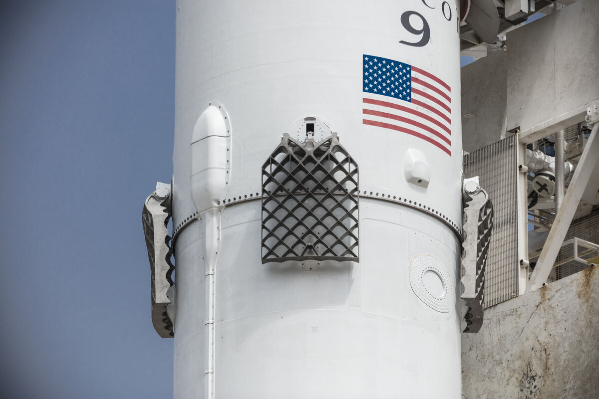
We built a pipeline that does exactly this: optimizing rocket grid fin geometry using Ansys SpaceClaim for CAD, a custom mesh converter, and PyMAPDL for structural analysis. The optimizer sees a single differentiable function, even though the underlying gradient strategies (analytical adjoint, finite differences, and JAX automatic differentiation) are completely different at every stage.
.jpg)
The pipeline
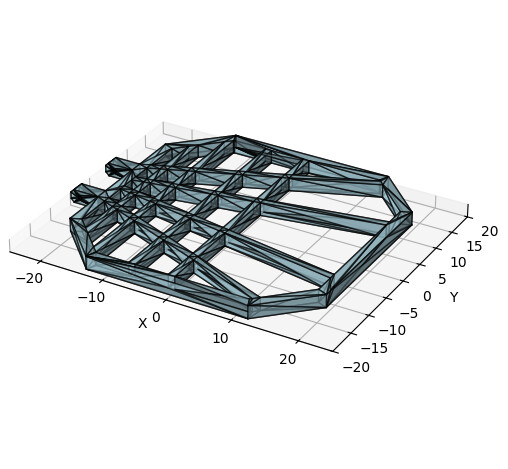
Each grid fin has 8 bars defined by start and end angular positions, giving us 16 design parameters. SpaceClaim generates the geometry, which gets converted to a signed distance field on a regular grid. PyMAPDL then solves the linear elasticity problem and returns compliance, a measure of how much the structure deforms under load. Lower compliance means a stiffer fin.
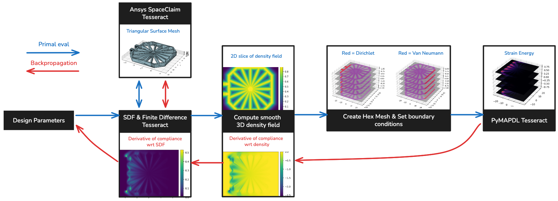
These tools don’t naturally fit together. SpaceClaim runs on Windows with a commercial license. PyMAPDL has its own dependency tree. The optimization logic and glue code run in JAX on Linux. We wrapped each step as a Tesseract: the SDF converter and PyMAPDL run as containerized images on Linux, while SpaceClaim runs directly on the Windows host via tesseract-runtime serve (since it needs the local Ansys installation). All three expose the same API regardless of deployment mode, and Tesseract-JAX composes them into a single callable pipeline.
None of this is specific to Ansys. We also ran the same optimization with PyVista for geometry and JAX-FEM as the solver. The Tesseract interfaces stayed the same — only the containers changed.
Getting gradients through
The trickiest part of this setup is differentiation. We need gradients of compliance with respect to the 16 bar parameters, but the gradient computation is different at every stage:
PyMAPDL computes gradients via an analytical adjoint. The solver already knows its own structure, so we can derive sensitivities directly from the stiffness matrix.
The SDF converter uses finite differences, wrapping the SpaceClaim Tesseract to perturb its inputs. SpaceClaim is a black box with no derivative information, so perturbation is the only option. This makes the SDF converter a higher-order Tesseract: a Tesseract that calls another Tesseract to compute its own gradients.
The density mapping and glue code between components use JAX automatic differentiation, since these are pure array operations where AD is straightforward.
Tesseract’s differentiation endpoints (Jacobian, JVP, VJP) provide a common interface across all three strategies. Tesseract-JAX chains them together so the optimizer sees a single differentiable function. This is the core idea: each component uses whatever differentiation strategy makes sense for it, and Tesseract handles the composition.
What the optimizer found
We ran Adam (learning rate 0.01, 80 iterations) from two starting points: a regular grid and a random bar arrangement.
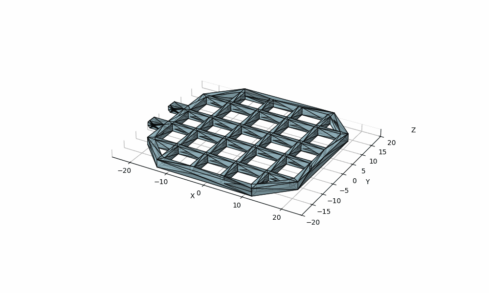
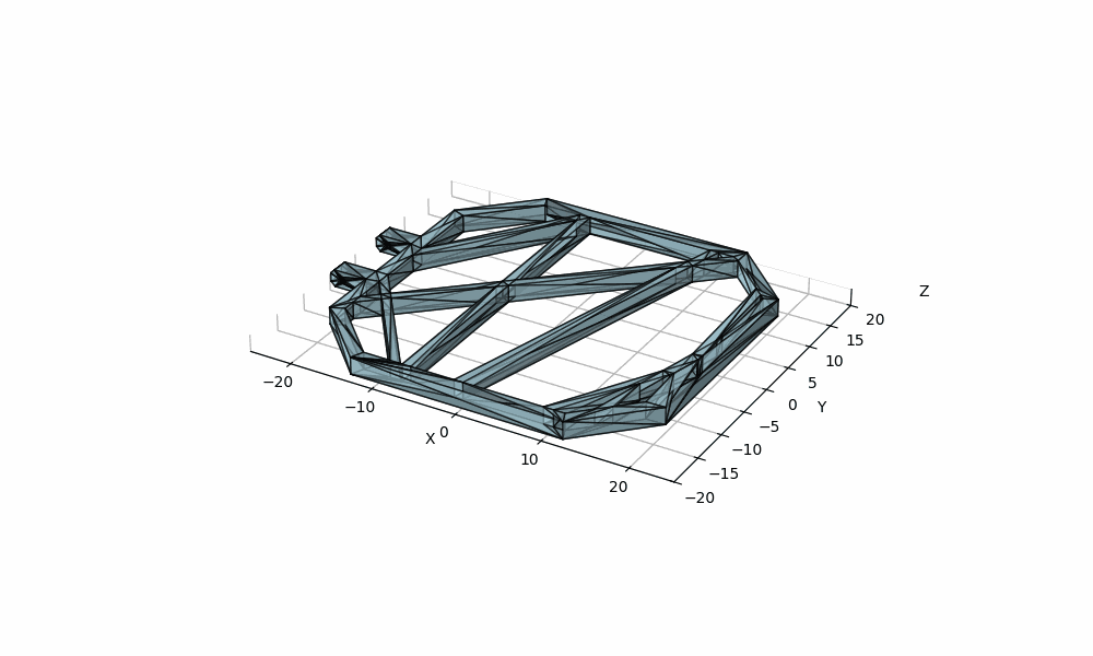
Both runs converged to similar topologies, which is a good sign that the optimizer isn’t just stuck in a local minimum. Three structural patterns emerged: bars organized into roughly orthogonal members, lateral bars angled diagonally to create direct load paths to the attachment points, and longitudinal bars clustered near the root where strain energy is highest.
The catch is that the raw optimized geometries are asymmetric and impractical to manufacture.
From optimizer output to a real design
Rather than using the optimizer’s output directly, we used it to inform a hand-designed geometry that incorporates the three structural patterns while enforcing symmetry and manufacturability.
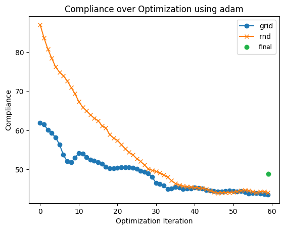
Running this geometry back through the pipeline gave a compliance of 49.8, 24% stiffer than the regular grid baseline at the same mass. It doesn’t match the unconstrained optimum, but it’s a practical design informed by what the gradients revealed about where material matters most.
Reflections
The main bottleneck in this pipeline is SpaceClaim, which has significant per-call overhead. Each optimization iteration takes on the order of minutes, so the full 80-iteration run takes a few hours. That’s acceptable for a design exploration study, but for tighter iteration loops, the PyVista + JAX-FEM variant runs much faster.
The broader pattern here extends well beyond structural optimization. Any workflow where you chain tools that differ in language, OS, licensing, or differentiation capability is a candidate for the same approach. The constraint that each component must expose a derivative endpoint through a common interface turns out to be a mild one — most solvers already have some notion of sensitivities, even if they don’t expose it as a clean API. Tesseract just gives those sensitivities a uniform shape.
If you want to dig into the details, the full technical writeup covers the methodology, and the demo code is ready to reproduce.
Tesseract is a free, open-source framework for differentiable scientific computing. pip install tesseract-core.
Docs · Demos · GitHub · Forum